5.3.23. Duct source option

To handle a very long neutron guide in a neutron spectroscopic facility, a duct source option that generates a special source was developed. Assuming an isotropic source, the current in a long beam line is inversely proportional to the square of the distance from the source position because of the solid-angle relation. This means that the current hitting the beam-line wall, called the wall current, becomes, for example, six orders of magnitude smaller at 100 m than at 1 m. To improve statistics in such a situation, an option was introduced that changes particle weights so that the wall current of simulation particles becomes the same at any position in the beam line.

This duct source option is applied by specifying dom = -10 for cylindrical and rectangular sources with s-type = 1, 2. The parameters and their meanings are summarized below.

dom = -10: Duct source option. dl0 =: Distance from the beam-line start point z0 [cm]. dl1 =: Distance from z0 to the start point of the duct source [cm]. dl2 =: Distance from z0 to the end point of the duct source [cm]. dpf =: Fraction of particles passing through dl2. drd =: Radius of the beam line [cm] for s-type = 1, cylinder. dxw =: X size of the beam line [cm] for s-type = 2, rectangular solid. dyw =: Y size of the beam line [cm] for s-type = 2, rectangular solid.

The beam-line shape is assumed to be cylindrical for s-type = 1 and rectangular for s-type = 2. It is also assumed that z1 = z0 and dir = 1. The latter indicates the beam-line direction. To change this, use trcl. Source particles are generated at z0, inside r0 for s-type = 1, or inside x0, x1, y0, y1 for s-type = 2.

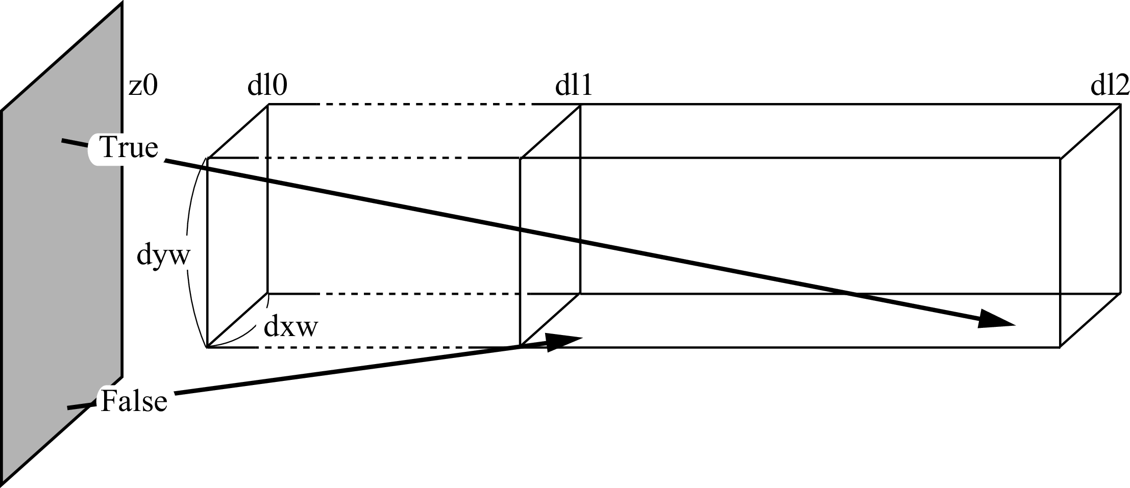
Fig. 5.3.10 Schematic view of the rectangular duct source

The source-particle direction is determined from the position where the particle hits the duct. The wall position is determined so that particles hit the duct uniformly between dl1 and dl2. Then, particle weights are determined assuming an isotropic distribution. The overall normalization constant is normalized by the number of particles passing through the duct at dl0 among the particles generated at z0 within the same area as the duct area at dl0. Usually, when the entire source region is visible from the duct wall between dl0 and dl2, this normalization constant is 1. If the source region at z0 is larger than the duct area at dl0, particles entering the duct from the larger region at z0 are not included in the normalization of source particles. This means that particles entering the duct from a region larger than the duct area at z0 increase the current in the duct without changing the normalization constant. This duct source assumes that the angular distribution at the source position is uniform over the solid angle of the duct area in the beam-line direction.

Next, simple examples are shown. The first example assumes a rectangular beam line, and the source size is the same as the guide cross section. The duct source section is

Listing 5.3.4 Example of duct source option (1)

   1:   [ Source ]
   2:
   3:   set: c1[200]    $dl0
   4:   set: c2[500]    $dl1
   5:   set: c3[5000]   $dl2
   6:   set: c4[5.0]    $x*2 at z0
   7:   set: c5[5.0]    $y*2 at z0
   8:   set: c10[5.0]   $dxw
   9:   set: c20[5.0]   $dyw
  10:   set: c30[0.001] $dpf
  11:
  12:   s-type = 2
  13:   proj   =  neutron
  14:   e0     =  20.0
  15:   x0     = -c4/2
  16:   x1     =  c4/2
  17:   y0     = -c5/2
  18:   y1     =  c5/2
  19:   z0     =  0.0
  20:   z1     =  0.0
  21:   dir    =  1.0
  22:   phi    =  0.0
  23:
  24:   dom = -10
  25:   dl0 = c1
  26:   dl1 = c2
  27:   dl2 = c3
  28:   dxw = c10
  29:   dyw = c20
  30:   dpf = c30

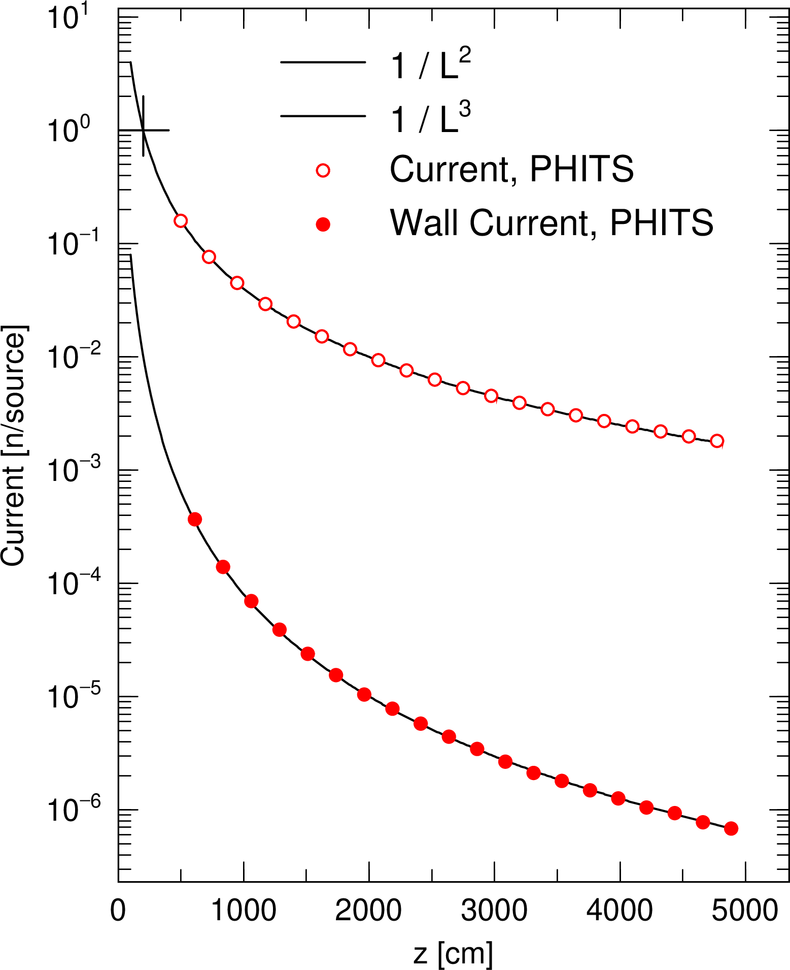
Fig. 5.3.11 Example of duct source option 1

The next example changes the size of the source region.

Listing 5.3.5 Example of duct source option (2)

   1:   [ Source ]
   2:
   3:   set: c1[200]    $dl0
   4:   set: c2[500]    $dl1
   5:   set: c3[5000]   $dl2
   6:   set: c4[10.0]   $x*2 at z0
   7:   set: c5[10.0]   $y*2 at z0
   8:   set: c10[5.0]   $dxw
   9:   set: c20[5.0]   $dyw
  10:   set: c30[0.001] $dpf
  11:
  12:   s-type = 2
  13:   proj   =  neutron
  14:   e0     =  20.0
  15:   x0     = -c4/2
  16:   x1     =  c4/2
  17:   y0     = -c5/2
  18:   y1     =  c5/2
  19:   z0     =  0.0
  20:   z1     =  0.0
  21:   dir    =  1.0
  22:   phi    =  0.0
  23:
  24:   dom = -10
  25:   dl0 = c1
  26:   dl1 = c2
  27:   dl2 = c3
  28:   dxw = c10
  29:   dyw = c20
  30:   dpf = c30

As shown in the following figure, in this example both the current and wall current increase. This increase indicates the contribution from the part of the source region larger than the duct. Therefore, this option can automatically treat contributions from the margin region of the source.

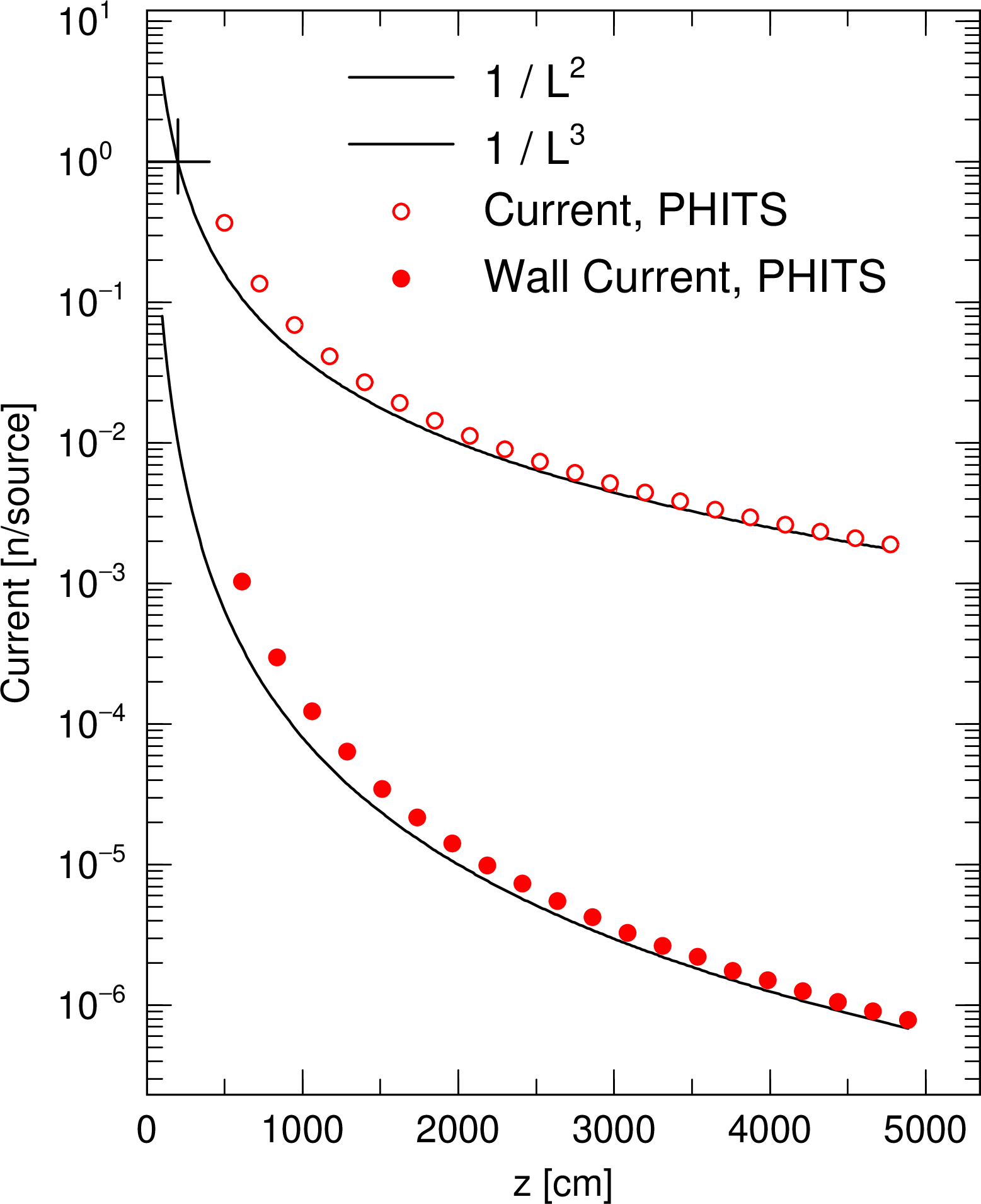
Fig. 5.3.12 Example of duct source option 2