6. General format of tally sections
PHITS has the following tally functions.
name |
explanation |
|---|---|
[t-track] |
Particle fluence in a certain region. |
[t-cross] |
Particle fluence crossing at a certain surface. |
[t-point] |
Particle fluence at a certain point. |
[t-deposit] |
Deposit energy in a certain region. |
[t-deposit2] |
Deposit energies in certain two regions. |
[t-heat] |
Heat generation in a certain region. (Not recommended [1] ) |
[t-yield] |
Production yield of residual nuclei. |
[t-product] |
Produced particles from source or nuclear reactions. |
[t-dpa] |
Displacements per atom (DPA). |
[t-let] |
Track length or dose as a function of LET. |
[t-sed] |
Energy deposition distribution in microscopic region. |
[t-time] |
Time dependent tally. |
[t-interact](formerly named [t-star]) |
Number of interactions occurred in specified regions. |
[t-dchain] |
Residual nuclide yields (in combination with DCHAIN). |
[t-wwg] |
Output parameters for [weight window]. |
[t-wwbg] |
Output parameters for [ww bias]. |
[t-volume] |
Automatic calculation of region volume. |
[t-userdefined] |
Any quantities that user defined. |
[t-gshow] |
2D geometry visualization. |
[t-rshow] |
2D geometry visualization with physical quantities. |
[t-3dshow] |
3D geometry visualization. |
[T-4Dtrack] |
Particle track files for displaying particle tracks in PHIG-3D. |
Common parameters used in these tallies are described below.
6.1. Mesh type
In the tallies shown in Table 6.1, region mesh (reg), r-z scoring mesh (r-z), and xyz scoring mesh (xyz) can be used for the mesh type of the tallying area. Additionally, tetrahedral mesh (tet) can be used for [t-track], [t-deposit], [t-yield], [t-product], [t-dpa], and [t-dchain].
One mesh should be specified like:
mesh = reg
6.1.1. Region mesh
The region mesh defined by the cell number can be written as follows. The reg= line must be the next effective input line after mesh=reg, where blank lines and comment lines are skipped. No other tally parameter can be written between mesh=reg and reg=.
mesh = reg
reg = 1 2 { 3 - 5 } all
Each cell number should be separated by blank. In the format { n1 - n2 } (n1 is smaller than n2), you can specify regions from n1 to n2. 3 - 5 in the above example means 3 4 5 . When you set all, all defined regions are separately specified.
Some regions can be combined by using ( ) .
mesh = reg
reg = ( 1 2 )  ( { 3 - 5 } )  ( all )
Specification of ( 1 2 ) gives a sum of tally results in the cell numbers 1 and 2. In the case of ( { 3 - 5 } ) , a sum of tally results in the cell numbers 3, 4, and 5 can be obtained. Note that you cannot specify like ( n1 - n2 ) . When you set (all) , you can obtain a sum of tally results in all defined regions. A new cell number of the combined region is given automatically starting from 1000001. The cell number is output in the echo part of the tally file, and is used when a volume of the region should be defined in a volume subsection, which will be mentioned in the next section.
When a geometry is defined using universe or lattice function, the geometry has repeated structures including several universes. A level structure is indicated by <, and the definition must be closed by ( ).
mesh = reg
reg = ( 301 < 101[0 0 0] )
This example refers to the geometry of Listing 5.6.9 in the [cell] section. The description above means cell number 301 in cell 101 at the lattice coordinate \((0,0,0)\) (see Section 5.6.4 for the lattice coordinate). You can specify a lattice coordinate by [ ] after the cell number corresponding to the lattice structure. Therefore, you can obtain a result of the cell number 301 included in a cell other than that at the lattice coordinate (0,0,0). When you specify some lattice coordinates separately, you can use the following format with commas: 101[-1 -1 0, 1 -1 0, 0 0 0] . Furthermore, when you use the format 101[-1:1 -1:1 0], you can tally nine results at lattice coordinates \((i,j,k)\) in the region \(-1 \le i \le 1\), \(-1 \le j \le 1\), \(k=0\). Note that this format gives the nine results individually. If you want a sum of the results, please use ( ) as in ( 301 < (101[-1:1 -1:1 0]) ). The style ( ) in one level can be used to combine some regions. When you specify ( u=3 < 101[0 0 0] ) , PHITS internally expands all cells included in u=3 . For example, in the case that two cell numbers 301 and 302 are included in u=3 , the above expression means reg= ( 301 < 101[0 0 0] ) ( 302 < 101[0 0 0] ) . You can use reg=all to specify all defined regions even in the case of the lattice structure, but cells other than in the bottom level are not considered.
6.1.1.1. Definition of the region and volume for repeated structures and lattices
See next example.
1:        mesh = reg
2:        reg = (all)
3:              ({ 201 - 205 })
4:              ( 161 < 160[1:2 3:6 1:1] )
5:              ( (201 202 203 204) < (161 162 163 ) )
6:              ( ( 90 100 ) 120 < 61 ( 62 63 ) )
As shown in the example above, the values of reg= can be written across multiple lines without using the line-connection symbol ( \ ). In this case, the values continue to be read as part of the reg= list until the next keyword (volume in this example) appears.
This region mesh definition is echoed as:
 1:        mesh =  reg            # mesh type is region-wise
 2:         reg = ( all ) ( { 201 - 205 } ) ( 161 < 160[ 1:2 3:6 1:1 ] ) ( (
 3:               { 201 - 204 } ) < ( { 161 - 163 } ) ) ( ( 90 100 ) 120 < 61
 4:               ( 62 63 ) )
 5:        volume                 # combined, lattice or level structure
 6:        non   reg      vol     # reg definition
 7:         1  10001   8.1000E+01 # ( all )
 8:         2  10002   5.0000E+00 # ( { 201 - 205 } )
 9:         3  10003   1.0000E+00 # ( 161 < 160[ 1 3 1 ] )
10:         4  10004   1.0000E+00 # ( 161 < 160[ 2 3 1 ] )
11:         5  10005   1.0000E+00 # ( 161 < 160[ 1 4 1 ] )
12:         6  10006   1.0000E+00 # ( 161 < 160[ 2 4 1 ] )
13:         7  10007   1.0000E+00 # ( 161 < 160[ 1 5 1 ] )
14:         8  10008   1.0000E+00 # ( 161 < 160[ 2 5 1 ] )
15:         9  10009   1.0000E+00 # ( 161 < 160[ 1 6 1 ] )
16:        10  10010   1.0000E+00 # ( 161 < 160[ 2 6 1 ] )
17:        11  10011   4.0000E+00 # ( ( { 201 - 204 } ) < ( { 161 - 163 } ) )
18:        12  10012   2.0000E+00 # ( ( 90 100 ) < 61 )
19:        13  10013   1.0000E+00 # ( 120 < 61 )
20:        14  10014   2.0000E+00 # ( ( 90 100 ) < ( 62 63 ) )
21:        15  10015   1.0000E+00 # ( 120 < ( 62 63 ) )
In the input, only 5 regions appear to be defined, but in the input echo, 15 regions are defined for the tally. In this input echo, region numbers are defined automatically starting from 10001, and the volume of each cell is set to 1 because there is no [volume] definition.
The details of the 15 regions appearing in the volume description of this input echo are explained below.
First, for ( all ), 81 cells are defined in the bottom level, so the volume of ( all ) is set to 81. If the volume of the cell is defined correctly in the [volume] section, you do not need to define the volume here again.
Next, for ( { 201 - 205 } ), this combined region has volume 5 in the echo, since this combined region has 5 cells at the bottom level. This also does not need to be re-defined here if the volume is set in the [volume] section.
For ( 161 < 160[1:2 3:6 1:1] ) , the region 161 is included as a lattice in region 160. In this expression in the lattice coordinate system, 8 lattices of region 160 from 1 to 2 in the \(i\) direction, 3 to 6 in the \(j\) direction, and 1 in the \(k\) direction are used for the tally. In the echo, the number of regions at the bottom level is shown as 1. In this case, you have to specify the volume yourself using the volume definition below.
For ( (201 202 203 204) < (161 162 163 ) ), some regions are defined at each level, but these are all enclosed by ( ), so this means one region as a whole. In this case, the volume given by the echo is not correct, so set the volume manually using the volume definition below.
For ( ( 90 100 ) 120 < 61 ( 62 63 ) ), there are two independent regions at each level, so 4 regions are defined here. In this case, the volume given by the echo is also not correct, so set the volume manually in the [volume] section.
You can set volume as below.
mesh = reg
reg = 1 2 3 4 ( 5 < 12 ) ( {13 - 17} )
volume
  reg       vol
    1       1.0000
    2       5.0000
    3       6.0000
    4       1.0000
10001       6.0000
10002       5.0000
In the above example, region numbers from 1 to 4 are set normally, but regions ( 5 < 12 ) and ( {13 - 17} ) have numbers 10001 and 10002. These large values are given automatically in the input echo. You can see and copy these settings from the input echo.
If you want to change the order of region number (reg) and volume (vol), set as vol reg . You can use the skip operator non .
In the input echo, numbered entry is given in non column. When axis=reg, the numbered entry is used as the value of the x-axis.
6.1.2. r-z mesh
When you use the r-z scoring mesh, first, offsets for x and y coordinate of the central axis of cylinder can be defined as:
mesh = r-z
x0 = 1.0
y0 = 2.0
This can be omitted.
Then, define r and z mesh as:
mesh   = r-z
r-type = [1-5]
..........
..........
z-type = [1-5]
..........
..........
Mesh definition is described in Section 6.6.
You can add \(\theta\) degree of freedom in r-z mesh of [t-track] tally. You can use a-type mesh definition to specify \(\theta\) of r-z mesh in the same manner as in the other angle mesh cases. However, the maximum angle of \(\theta\) mesh is restricted 360 degree ( \(2\pi\) ) in this case. You can obtain the \(\theta\) dependence of results of [t-track] tally by setting axis=rad or axis=deg . The rad represents the \(\theta\) in radian, while deg in degree.
6.1.3. xyz mesh
When you use the xyz scoring mesh, set x, y, and z mesh as:
mesh   = xyz
x-type = [1-5]
..........
..........
y-type = [1-5]
..........
..........
z-type = [1-5]
..........
..........
Mesh definition is described in Section 6.6.
6.1.4. tet mesh
This mesh is applicable only when tetrahedron geometry described in Section 5.6.5.4 is used in the geometry and is active only in [t-track], [t-deposit], [t-yield], [t-product], and [t-dpa] tallies. When you use the tet scoring mesh, the cell number of the rectangular box where the tetrahedron geometry is implemented needs to be specified following the mesh definition, as shown below:
mesh   = tet
reg   = 100
The physical quantities specified in the tally will be scored in all tetrahedrons separately. Extraction of some tetrahedrons can be achieved by specifying the region in hierarchical universe region format as:
reg = ( 201 202 < 101 )
where 201 and 202 are the cells corresponding to the universes of the tetrahedron geometry specified in cell 101 (Example Listing 5.6.15). The physical quantities for tetrahedrons belong to those universe regions are separately tallied. Additionally only the universe region specification
reg = 201
is also possible. For more than one universe region, bracket specification such as (201 202) is necessary. These universe region specifications are valid when only one tetrahedron geometry is included in the PHITS input. Summation of tetrahedrons is possible using region mesh (mesh=reg) by selecting the universe region. It should also be noted that the volume of a tetrahedron is simply computed from the coordinates of the nodes, and thus incorrect quantities may be obtained when the tetrahedron geometry is clipped out through the use of nested universe and fill structures. In such a case, region mesh (mesh=reg) should be used instead.
6.2. Energy mesh
Energy mesh begins as:
e-type = [1-5]
..........
..........
The unit is MeV (however, when particle energy is defined, it can be switched to MeV/n or nm by iMeVperN or e-unit). e1-type and e2-type are also used in [t-deposit2] tally. Mesh definition is described in Section 6.6.
6.3. LET mesh
LET mesh begins as:
l-type = [1-5]
..........
..........
The unit is keV/um. Mesh definition is described in Section 6.6.
6.4. Time mesh
Time mesh is defined as:
t-type = [1-5]
..........
..........
The unit is nsec. Mesh definition is described in Section 6.6.
6.5. Angle mesh
Angle mesh in cross tally is defined as:
a-type = [1, 2, -1, -2]
..........
..........
If a-type is defined by positive number, this mesh denotes cosine mesh. If a-type is defined by negative number, the mesh denotes angle mesh. Mesh definition is described in Section 6.6.
6.6. Mesh definition
There are 8 kinds of mesh definition as e-type, t-type, x-type, y-type, z-type, r-type, a-type, l-type . The format is common for every mesh types. So only the e-type definition is described below. For other types, replace e into t, x, y, … and a. For example, replace ne as nt, nx, ny, … , na , emin as tmin, xmin, ymin, … , amin , and so on.
In the defined mesh, emin itself is included in the minimum bin, while emax itself is not included in the maximum bin.
6.6.1. Mesh type
You can use 5 kinds of mesh type as shown below.
mesh type |
explanation |
|---|---|
1 |
Give number of groups and mesh points by data. |
2 |
Give number of groups, minimum and maximum values. Mesh is divided equally by linear scale. |
3 |
Give number of groups, minimum and maximum values. Mesh is divided equally by log scale. |
4 |
Give mesh width, minimum and maximum values. Mesh points are given by linear scale. Number of groups is set automatically as resulting maximum value becomes same with given value, or takes larger value with small excess as possible. |
5 |
Give minimum and maximum values and log value of mesh width. Mesh points are given by log scale. Number of groups is set automatically as resulting maximum value becomes same with given value, or takes larger value with small excess as possible. |
It is noted that you can use only 1, 2 (-1, -2) mesh types in a-type definition.
Only when [t-cross] and z-type=1 , nz=0 can be set with only one data. This setting provides only one tally surface of z=(data).
Each mesh type format is shown in followings.
6.6.2. e-type = 1
When you use e-type=1 , set number of group, then numerical data as:
e-type = 1
  ne = ngroup
    data(1) data(2) data(3) data(4)
    data(5) data(6) data(7) data(8)
    .........
    .........
    data(ngroup+1)
You can use multi lines without any symbols for line connection.
6.6.3. e-type = 2, 3
When you use e-type=2,3 , set number of group, minimum value, and maximum value as:
e-type = 2, 3
  ne = ngroup
  emin = minvalue
  emax = maxvalue
ngroup represents the number of energy groups. The mesh is defined by equally dividing the range from the minimum value (minvalue) to the maximum value (maxvalue) either linearly (when e-type = 2) or logarithmically (when e-type = 3).
6.6.4. e-type = 4
When you use e-type=4, set mesh width, minimum value, and maximum value as:
e-type = 4
  edel = width
  emin = minvalue
  emax = maxvalue
The range from the minimum value (minvalue) to the maximum value (maxvalue) is divided linearly using width as the mesh size.
6.6.5. e-type = 5
When you use e-type=5, set mesh width, minimum value, and maximum value as:
e-type = 5
  edel = widthlog
  emin = minvalue
  emax = maxvalue
In this case, the mesh width represents the width in the logarithmic scale. That is, widthlog is defined as \(\log\left(\frac{M_{i+1}}{M_i}\right)\) .
6.7. Other tally parameters
6.7.1. part parameter
You can define particles as
part = proton neutron pion+ 3112 208Pb
or
part = proton
part = neutron
part = pion+
part = 3112
part = 208Pb
See Section 4.7 for particle identification. You can also use the kf code number.
If you define all particles as
part = all
If you want to tally some particles as a group, you can use ( ) as the following. The maximum number inside the ( ) is 6. One caution to use kf code number inside ( ) is that a space before ) is required after the last kf code number.
part = ( proton neutron ) all pion+ 3112 208Pb
In this case, as the first group, the sum of proton and neutron contribution is tallied, the second is the sum of all. 5 groups of the particle are printed out in this tally.
For nucleus, you can use the expression like 208Pb and Pb. The latter case, Pb, denotes all isotopes of Pb.
By setting a minus sign before the particle name, you can tally the results without contribution from the specified particle. ( ) is required to use kf code number and the minus sign is needed before ( ) . You can also tally the results without contributions from a group of particles by using ( ) . The minus sign should be placed before ( ) after grouping the particles. The use of a minus sign to subtract a contribution is not allowed inside ( ).
part = -proton -(proton alpha) -(2112) -(11 -11)
The first specification gives a result without proton contribution, the second gives a result without proton and alpha contributions, the third gives a result without neutron (2112) contribution, and the fourth gives a result without electron (11) and positron (-11) contributions.
6.7.2. axis parameter
X axis value for output is described here. There are many kinds of axis, depending on the tally type and mesh type:
eng,  reg,  x,  y,  z,  r,  t,  xy,  yz,  zx,  rz,
cos,  the,  mass,  charge,  chart,  dchain,
let, t-eng, eng-t, t-e1, e1-t, t-e2, e2-t, e12, e21
axis = eng
You can set multiple axis per one tally by
axis = eng x y
or
axis = eng
axis = x
axis = y
If you define multiple axes, output results are written in different files. So you need to specify multiple output files as shown in the next subsection when multiple axes are defined.
It should be noted that you can define only one axis in a [t-yield] section from ver. 2.50. This restriction was implemented to calculate statistical uncertainties correctly. If you want to define several axes in the [t-yield] tally, you have to set the corresponding number of [t-yield] sections in an input file.
6.7.3. samepage parameter
This parameter specifies the type of data to be displayed on the same page of the image output file. The parameter must be selected from those listed in the axis parameter. The default is part , in which case the results for multiple particles specified in the part parameter are output on the same page. The values of samepage and axis should NOT be the same. Note that when the number of data bins specified in samepage exceeds 20, the eps file only shows the results of bins 1 through 20. Not available for [t-yield] tally and some others.
6.7.4. file parameter
The format to define name of output file is,
file = file.001 file.002 file.003
Note that the file name should not have the extension of .eps or .vtk. As described before, when you set multiple axis , set output files for each axis like following example.
file = file.001
file = file.002
file = file.003
6.7.5. resfile parameter
Specify the name of the tally file output from the previous calculation to determine the random number to be used in the restart calculation. The format is shown below.
resfile = file.out
If you specify the file in a different directory than the input file, specify it as a relative or absolute path. Even if several resfile parameters are set in a tally section, only the earliest one is used. resfile is set to file by default. In this case, results of the past tally are overwritten.
6.7.6. unit parameter
Set output unit as
unit = number
The unit number and its meanings are described in each tally explanation.
6.7.7. factor parameter
You can use the format below to set the normalization factor.
factor = value
If factor is positive, all the results are multiplied by this factor. If factor is negative (e.g. -c), all the results are scaled so that the maximum becomes c. When you use the [t-gshow] tally, this factor defines the line thickness instead.
6.7.8. output parameter
Set output type as
output = name of output
Details are described in each tally explanation.
6.7.9. info parameter
This option defines whether detailed information is output or not. Set 0 or 1 as
info = 0, 1
6.7.10. title parameter
This option is for title as
title = title of the tally
It is omitted, and in this case, default is used.
6.7.11. ANGEL parameter
In order to add ANGEL parameters in tally output, define as
angel = xmin(1.0) ymin(1.3e-8)
Defined parameters are converted to the ANGEL format as
p: xmin(1.0) ymin(1.3e-8)
These parameters change the minimum of the horizontal and vertical axes, respectively. The main ANGEL parameters are shown in Table 13.1.1. Please see the ANGEL manual for more details.
6.7.12. SANGEL parameters
This parameter can be used to insert all ANGEL parameters into tally output files, unlike the usual ANGEL parameter, which can specify only ANGEL parameters defined by p:. For example, by defining infl: parameter for ANGEL, the tally output file can include an external file containing experimental data, and both calculated results and the experimental data can be plotted in a figure.
The SANGEL parameter can be set using the format sangel= number of parameter lines, and then writing that number of lines to define the ANGEL parameters. An example with sangel is as follows.
sangel = 2
infl:{exp.dat}
w: ($theta=$ 0 deg) / X(10) Y(100)
Here, exp.dat is a data file of the experimental data.
The data can be shown on the figure of the tally result.
By using w: parameter, the comment theta=0 deg can be put at the coordinate of X=10, Y=100 in the figure.
From version 3.31 onward, infl in sangel cannot be used by default. If you need to use it, add $RWT=0 before the first section begins.
6.7.13. 2d-type parameter
When you define 2 dimensional output as axis=xy , you must set this 2d-type option as
2d-type = 1, 2, 3, 4, 5, 6, 7
These 2d-type values determine the data arrangement format.
2d-type = 1, 2, 3, 6, 7
Data are written in the format below (the example is written in Fortran style).
( ( data(ix,iy), ix = 1, nx ), iy = ny, 1, -1 )
10 data are written in a line. Also a header for the ANGEL input is inserted. The ANGEL header is inserted by 2d-type=1 for contour plot, 2d-type=2 for cluster plot, 2d-type=3 for color plot, 2d-type=6 for cluster and contour plot, 2d-type=7 for color and contour plot.
2d-type = 4
Data are written in the format below.
do iy = ny, 1, -1
  do ix = 1, nx
    ( x(ix), y(iy), data(ix,iy) )
  end do
end do
3 data of x(ix), y(iy) and data(ix,iy) are written in a line.
2d-type = 5
Data are written in the format below.
y/x  ( x(ix), ix = 1, nx )
do iy = ny, 1, -1
  ( y(iy), data(ix,iy), ix = 1, nx )
end do
nx+1 data are written in a line, and total ny+1 lines. It is useful in tabular software such as Excel.
6.7.14. gshow parameter
This option can be used in all tallies except [t-gshow] and [t-rshow]. If you set gshow option with xyz mesh, xy, yz, or xz axis, and 2d-type=1,2,3,6 or 7, ANGEL can create a graphical plot with region boundary and material name, or region name, or lattice number on the two dimensional output. You can also obtain graphical plots directly from the PHITS calculation by the epsout option.
gshow = 0, 1, 2, 3, 4, 5
In the above example, 0 means no gshow option, 1 means gshow with region boundary, 2 means gshow with region boundary and material name, 3 means gshow with region boundary and region name, 4 means gshow with region boundary and lattice numbers, and 5 means gshow with material color. When you increase the resolution of the plot by resol parameter, the indication of region name, material name and lattice number on the graph are sometimes disturbed. In this case, you should increase the mesh points instead of resol .
You can see your geometry plot without transport calculation by setting icntl=8 in the [parameters] section together with this gshow option. You should check whether the regions are correct and whether the xyz mesh resolution is appropriate before a long calculation.
6.7.15. rshow parameter
You can use rshow parameter in all tallies except for [t-cross] and [t-gshow] tallies. This option is available with mesh=reg or tet , and axis=xy, yz, zx . This option makes a two dimensional plot in which each region or tetrahedral element is colored with the amount of the output value in the region or tetrahedral element, respectively. And region boundaries, material name, or region name numbers are also displayed. The xyz mesh definition is required after this rshow parameter.
rshow =  1, 2, 3
x-type = [2,4]
  ..........
  ..........
y-type = [2,4]
  ..........
  ..........
z-type = [2,4]
  ..........
  ..........
rshow=0 means no rshow option, 1 means rshow with region boundary, 2 means rshow with region boundary and material name, 3 means rshow with region boundary and region name numbers. If rshow=0, xyz mesh definition is not required, and should be commented out. When you increase the resolution of the plot by resol parameter, the indication of region name, material name and lattice number on the graph are sometimes disturbed. In this case, you should increase the mesh points instead of resol. Please note that without gslat option, the boundaries between the same material (rshow=2) or same cell (rshow=3) regions will not be shown and inaccurate value may be displayed for each region or tetrahedron. Therefore, use of gslat=1 in addition is recommended.
If you use the rshow option with reg mesh, there is no output for the values of each region. In this case, you cannot re-plot the figure because of no original data. When this rshow option is used, usually axis is set as xy, yz, and zx. But you should use in addition axis=reg or tet in order to save results into another file, for re-plotting. You can re-plot figures from saved data and [t-rshow] tally function.
You can execute this option without transport calculation by using icntl=10 in the [parameters] section. For icntl=10, PHITS makes a two dimensional plot for the tallies with reg mesh, xy, yz, zx axis and rshow = 1, 2, 3. In the figure, different colors are used for different materials. You should check whether the regions are correct and whether the xyz mesh resolution is appropriate before a long calculation.
6.7.16. x-txt, y-txt, z-txt parameter
If you want to change x, y, and z axis titles in the output figure, use these options. These titles cannot be defined in the ANGEL parameter.
x-txt = x axis title y-txt = y axis title z-txt = z axis title
6.7.17. volmat parameter
The volmat parameter corrects a volume where xyz mesh crosses region boundaries. This option is effective in the case that mesh is xyz, and the material parameter is defined. This corrected volume is calculated by the Monte Carlo method for specified material. volmat denotes the number of scanning parallel to x, y, and z axis respectively for the Monte Carlo calculation. So if you set too large volmat, the calculation takes long time. You need to take care of it. If volmat is given by negative value, all xyz mesh is scanned. If positive value, the scanning is not performed when 8 apexes of the mesh are included in the same material.
6.7.18. epsout parameter
If you set epsout=1, output file is treated by ANGEL automatically and an eps file is created. This eps file name is named by replacing the extension into .eps. With itall=1 setting, the eps file is created after every batch calculation. You can monitor the PHITS results in real time, by displaying the eps file.
6.7.19. counter parameter
You can make a gate to the tallying quantities by using the counter defined by [counter] section. Set minimum ctmin(i) and maximum value ctmax(i) for each counter. The i is the counter number from 1 to 3. By default, ctmin(i)=-9999, and ctmax(i)=9999. When multiple counters are specified, the common part of these terms is tallied.
In addition, you can make a gate to the tallying quantities by using the history-counter, which is the maximum counter value of all particles generated in one history, by setting chmin(i) and chmax(i) parameters.
Using this function, you can tally your interested events selectively by tracing back to the generation of their sources.
Please see /phits/sample/misc/history_counter for more details.
Note that the history-counter does not work in the batch variance mode (istdev=1).
Furthermore, this function does not work well when variance reduction method such as [weight window] is used or the event generator mode is not used.
6.7.20. resolution and line thickness parameters
You can increase the resolution of the region boundaries in the gshow, rshow, and 3dshow with keeping xyz mesh by resol. Default value is 1, it is same as xyz mesh resolution. If you set resol=2, the resolution becomes 2 times for each side. It is useful to draw smooth line for xyz mesh. Also you can obtain clear graphics by set resol larger for the 3dshow. Even if you set resol larger, memory usage is not changed.
The width shows the line thickness for gshow, rshow, and 3dshow. Default value is 0.5.
6.7.21. trcl coordinate transformation
By this trcl option, you can transform the coordinate of the r-z, and xyz mesh. There are two ways to define the transformation as below.
trcl = number
trcl = O1 O2 O3 B1 B2 B3 B4 B5 B6 B7 B8 B9 M
The first definition is to specify the transformation number defined in [transform] section. The next one is to define the transformation directly here with 13 parameters as same as in [transform] section. If the data are not written in a line, you can write them in multiple lines without the line sequential mark. But you need to put more than 11 blanks before data on the top of the sequential lines.
In the 3dshow tally, trcl can be used to transform the box. This will be explained in the [t-3dshow] tally section.
6.7.22. Particle information for Dump function
The dump parameter can be specified in the [t-track], [t-cross], [t-point], [t-deposit], [t-product], [t-dpa], [t-time], and [t-interact] tallies [2] to output detailed information for each tallied particle. After specifying the number of data items to be output via the dump parameter (positive for binary format, negative for ASCII data), the particle information ID numbers (see Table 6.7.1 ) are defined on the subsequent line.
At least two files are produced when the dump parameter is defined.
The standard tally results are written in text format to the file specified by the file parameter.
Simultaneously, the dumped particle information is written to a file named by appending _dmp before the extension of the specified filename.
In distributed-memory parallel computing, (NPE - 1) files are created, where NPE is the total number of Processing Elements (PEs).
A file is generated for each PE with its PE number appended to the end of the filename; each PE writes to and reads from its corresponding file only.
Note that the creation of dump files via this function and the event information output using the dumpall parameter are mutually exclusive and cannot be used simultaneously during shared-memory parallel computing
ID |
Symbol |
Description |
|---|---|---|
1 |
kf |
Kind of the current or produced particle (kf-code) |
2 |
x |
x-coordinate of the current or produced particle (cm) |
3 |
y |
y-coordinate of the current or produced particle (cm) |
4 |
z |
z-coordinate of the current or produced particle (cm) |
5 |
u |
x-component of the direction vector of the current or produced particle |
6 |
v |
y-component of the direction vector of the current or produced particle |
7 |
w |
z-component of the direction vector of the current or produced particle |
8 |
e |
Energy of the current or produced particle (unit depends on iMeVperN or e-unit ) |
9 |
wt |
Weight of the current or produced particle |
10 |
tm |
Time of the current or produced particle (ns) |
11 |
c1 |
Counter 1 value of the current or produced particle |
12 |
c2 |
Counter 2 value of the current or produced particle |
13 |
c3 |
Counter 3 value of the current or produced particle |
14 |
sx |
x-component of the spin vector of the current or produced particle |
15 |
sy |
y-component of the spin vector of the current or produced particle |
16 |
sz |
z-component of the spin vector of the current or produced particle |
17 |
name |
Collision number of the current or produced particle (for developers) |
18 |
nocas |
History number in the current batch |
19 |
nobch |
Batch number |
20 |
no |
Cascade ID in the current history (for developers) |
21 |
kf0 |
Kind of the past or parent particle (kf-code) |
22 |
x0 |
x-coordinate of the past or parent particle (cm) |
23 |
y0 |
y-coordinate of the past or parent particle (cm) |
24 |
z0 |
z-coordinate of the past or parent particle (cm) |
25 |
u0 |
x-component of the direction vector of the past or parent particle |
26 |
v0 |
y-component of the direction vector of the past or parent particle |
27 |
w0 |
z-component of the direction vector of the past or parent particle |
28 |
e0 |
Energy of the past or parent particle (unit depends on iMeVperN or e-unit ) |
29 |
wt0 |
Weight of the past or parent particle |
30 |
tm0 |
Time of the past or parent particle (ns) |
31 |
tv |
Tally value (the value added to the tally by the event) |
32 |
rec |
Reaction ID number (Category ID × 1000 + Sub-category ID, see Table 6.7.2 and Table 6.7.3 ) |
33 |
cel |
Region (cell) number at the current or produced particle coordinates |
34 |
mat |
Material number at the current or produced particle coordinates |
For example, if you define:
dump = 9
  1  8  9  2  3  4  5  6  7
The data will be output in binary format in the order of kf e wt x y z u v w . For tallies other than [t-product] and [t-interact], the tally value is calculated from the particle information of the current and the previous (past) steps; therefore, this information is output to IDs 1-17 and 21-30, respectively. In contrast, for [t-product] and [t-interact], the information for the particle produced after the reaction and its parent particle is output to IDs 1-17 and 21-30, respectively. However, if a particle is cut off or generated as a source, the information for IDs 1-10 and 21-30 will be identical.
In cases where output = deposit in [t-deposit] and MorP = prob in [t-interact], the tallying is performed at the end of each history rather than during particle transport. Consequently, information other than ID 18 (history number), 19 (batch number), and 31 (tally value = weight of the particle that first contributed to the event) cannot be output. These values are followed by the deposited energy or the number of interactions in each region. For instance, if you define:
dump = -3
  18 19 31
for [t-deposit] with output = deposit , the data will be output in ASCII format in a single line as nocas nobch tv [deposited energy in each region], separated by spaces. Note that even if multiple particles are specified in the part parameter, only the results for the first specified particle (which is forced to be all in [t-deposit]) are output. Furthermore, even if material or t-type are specified, only the total values are output.
The tally value output at ID 31 represents the value added to the tally result during the event. It is calculated by multiplying the current particle weight ( wt ) by the following factors: the distance between the current and past particles (track length) for [t-track], \(1/\cos\theta\) for [t-cross] with output = flux , the flux added to the tally point for [t-point], the deposited energy for [t-deposit], or the DPA value for [t-dpa]. For other tallies, the factor is 1. The reaction ID number output at Particle-information ID 32 is determined as Category ID x 1000 + Sub-category ID based on the IDs shown in Table 6.7.2 and Table 6.7.3 . For example, if the category is Nuclear Reaction and the sub-category is Elastic Scattering (MT=2), the reaction ID will be 2002.
Category ID |
Description |
|---|---|
0 |
Non-reaction events (particle transport, source generation, etc.) |
1 |
Particle decay |
2 |
Nuclear reaction |
3 |
Atomic interaction |
4 |
Interaction in track-structure mode |
Category ID |
Sub-category ID |
Description |
|---|---|---|
1 |
0 |
Particle decay |
2 |
MT number [4] |
Nuclear reaction. Sub-category is 0 for reactions not classified by MT numbers. |
3 |
0 |
Other atomic interactions |
3 |
1 |
Delta-ray production |
3 |
2 |
Atomic fluorescence X-ray production |
3 |
3 |
Auger electron production |
3 |
4 |
Bremsstrahlung production |
3 |
5 |
Photoelectric effect [5] |
3 |
6 |
Compton scattering |
3 |
7 |
Electron-positron pair production [6] |
3 |
8 |
Positron annihilation |
3 |
9 |
Rayleigh scattering and electron multiple scattering |
3 |
10 |
Optical photon interaction |
4 |
0 |
Other track-structure interactions |
4 |
1 |
Elastic scattering |
4 |
2 |
Ionization |
4 |
3 |
Electronic excitation |
4 |
4 |
Dissociative electron attachment |
4 |
5 |
Vibration excitation |
4 |
6 |
Phonon excitation |
4 |
7 |
Rotation excitation |
4 |
8 |
Plasmon excitation |
4 |
9 |
Electron capture |
4 |
10 |
Electron stripping |
6.8. Function to sum up two (or more) tally results
After version 2.74, PHITS has a function to sum up two (or more) tally results. There are two methods for sum up; one is to integrate the tally results considering the history number of each simulation, while the other is to add the tally results weighted by user defined ratios. The former can be used for the parallel calculation on computers in which MPI protocol is not installed. On the other hand, the latter is suit for the simulation with different source terms whose intensities cannot be fixed before the simulation, such as that for Intensity-Modulated Radiation Therapy (IMRT).
In order to use this function, you have to satisfy the following conditions:
icntl is set to 13 in [parameters] section.
The parameters for each tally results such as mesh, axis and part are identical to one another.
A sumtally subsection is defined in the tally section that outputs one of the summing up tallies. [7] [8]
The sumtally subsection is ignored when icntl parameter is not set to 13 in [parameters] section. [9]
Please see the ppt slides or sample input file in \phits\lecture\advanced\sumtally\ for details.
The sumtally subsection should be defined between the lines of sumtally start and sumtally end written in the tally section that outputs one of the summing up tallies. The set: definition is ignored in the sumtally subsection.
The parameters used in the sumtally subsection are summarized in Table 6.8.1.
name |
value |
description |
|---|---|---|
isumtally = |
1(default), 2 |
Summing up procedure. 1: Integration of tally results considering history number of each simulation. 2: Sum of tally results weighted by user defined ratios. |
nfile = |
Number |
Number of summing up files. |
(next line) |
filename value |
Summing up file name, weighted value. Sum of the weighted values is automatically normalized to sumfactor for isumtally=2. |
sfile = |
filename |
Output file name. |
sumfactor = |
(optional, D=1.0) |
Normalization factor. |
Users can use isumtally=1 to manually obtain the parallel calculation results.
For example, if you have one tally result result-1.out obtained with maxbch=10 and maxcas=100, and another tally result result-2.out obtained with maxbch=20 and maxcas=100, and if you would like to sum up the results to have same statistics as of maxbch=30 and maxcas=100, you have to write:
   1:  sumtally start
   2:  isumtally = 1        $(D=1) sumtally option, 1:integration, 2:weighted sum
   3:  nfile = 2            $ number of tally files
   4:     result-1.out  1.0
   5:     result-2.out  1.0
   6:  sfile = result-s.out $ file name of output by sumtally option
   7:  sumfactor = 1.0      $ (D=1.0) normalization factor
   8:  sumtally end
Using this sumtally subsection, you can obtain the results for maxcas=100 and maxbch=30.
Please be sure that the initial random seeds for calculating result-1.out and result-2.out should be different from each other, otherwise you would get biased results for certain random numbers.
The most recommended method for changing the initial random seed is to use irskip parameter.
The weighted value for each tally outputs are generally set to 1 for isumtally=1, unless you would like to change the weight of source particles.
The output file obtained from this sumtally section, result-s.out, can be used for restart calculation by setting istdev<0.
Note that the initial random seed in the last file of the summing up files is used.
For isumtally=2, the weighted summation of the tally results, \(\bar{X}\), is calculated by the following equation:
where \(F\) is the normalization factor defined by sumfactor, \(N\) is the number of summing up files defined by nfile, \(\bar{X}_j\) is the \(j\)-th tally results, \(r_j\) is the weighted value of \(j\)-th tally, and \(r\) is the sum of \(r_j\), that is, \(r=\sum_{j=1}^N r_j\). The uncertainty of the summation value, \(\sigma_X\), can be calculated by
where \(\sigma_{X_j}\) is the standard deviation of \(j\)-th tally results.
If you have two tally results result-l.out and result-r.out, and you would like to sum up them weighted by factors of 2.0 and 3.0, respectively, you have to write:
   1:  sumtally start
   2:  isumtally = 2        $(D=1) sumtally option, 1:integration, 2:weighted sum
   3:  nfile = 2            $ number of tally files
   4:     result-l.out  2.0
   5:     result-r.out  3.0
   6:  sfile = result-s.out $ file name of output by sumtally option
   7:  sumfactor = 5.0      $ (D=1.0) normalization factor
   8:  sumtally end
You can obtain the same results by using multi-source function, but it is more convenient to use sumtally subsection when you would like to change the weighted values for several cases.
It should be mentioned that the sum of the weighted values is automatically normalized to sumfactor for isumtally=2.
For example, in this case, we want to double result-l.out and triple result-r.out before summing them, so we set sumfactor to 5.
The output file obtained from this sumtally section, result-s.out, cannot be used for restart calculation.
6.9. Function to analyze two (or more) tally results
Unlike the function in the previous section, you can perform more complex calculations using two (or more) tally results through an anatally function. For example, you can calculate the biological dose for charged particle therapy taking into account the absolute values of the absorbed doses, or you can estimate the effect of a material density error on the calculated results as systematic uncertainties.
This function analyzes multiple tally results obtained from normal transport calculations. It works in two ways.
After performing the normal transport calculation manually, specify the resulting tally file to run the anatally function.
Using
autorunscript automatically run through usual transport calculations and anatally function.
The latter method is basically used to evaluate the systematic uncertainty. Although the former method can also be used for evaluation, the latter is more convenient for evaluating uncertainty by varying a large number of input values.
The Anatally function itself works by setting icntl=17 in the [parameters] section. However, the following conditions must be met.
Multiple tally results to be analyzed must be obtained with the same conditions regarding mesh, axis, part and the division number (bins) of energy, space, and so on.
A [anatally] section should be set with specifying the file names of the tally results to be analyzed.
An empty anatally subsection, consisting of only anatally start and anatally end, is defined in the tally section that outputs the tally results.
[anatally] section is available only when icntl=17.
In this case, two anatally subsections are needed in the [anatally] and usual tally sections.
The former subsection should contain the parameters of the anatally function, such as the file names of the tally results, while an empty subsection consisting only of anatally start and anatally end should be written in the latter subsection.
Note that when you use the autorun script shown in Section 6.9.2, you should set icntl=16, define the anatally subsection with information about the tally file names in the usual tally section, and not set [anatally] section.
Also note that, when running with icntl=17 (the anatally reprocessing run itself), for the empty anatally start/anatally end subsection set in a [t-track] or other usual tally section, the line right after anatally start must be anatally end. Inserting a comment line between them causes an error.
The anatally subsection should be defined between the lines of anatally start and anatally end. The set: definition is ignored in the anatally subsection.
The parameters used in the anatally subsection are summarized in Table 6.9.1. Note that parameters shown in the Extended statistical indicators section, such as ix, iy, iz, and ipart, which are available when itall=3, cannot be used when icntl=16,17.
name |
value |
description |
|---|---|---|
ianataldchain = |
(optional, D=0) |
Option for [t-dchain] tally.
0: Do not use tally result files of [t-dchain].
1: Use tally result files of [t-dchain].
Specifying filenames given as part parameters in the [t-dchain] section automatically handles the other output files for DCHAIN ( |
manatally = |
0, 1(default) |
Control parameter of anatally function.
0: user-defined anatally function.
Program written in |
nfile = |
Number |
Number of tally files. |
(next line) |
file name |
file name for analysis |
sfile = |
file name |
output file name |
   1:  [t-track]
          .........
          .........
   2:  anatally start
   3:  anatally end
          .........
          .........
   4:  [anatally]
   5:  anatally start     1
   6:  manatally = 0        $(D=1) anatally option, 0:user-defined anatally, 1:anova
   7:  nfile = 2            $ number of tally files
   8:     result-1.out
   9:     result-2.out
  10:  sfile = result-a.out $ file name of output by anatally option
  11:  anatally end     1
In this example, calculation of user-defined anatally function is used with result-1.out and result-2.out, which are output files of [t-track] obtained by usual transport calculations (icntl=0), and then its result is outputted in result-a.out.
The numbers 1 written in the lines of anatally start and anatally end are anatally subsection ID.
This ID corresponds to the order of the tally section in the PHITS input file.
You have to set the order of the tally section including anatally subsection.
For example, if one more tally section is defined before the [t-track] in the first line, the ID should be set 2 in the [anatally] section.
6.9.1. User-defined anatally function
The user-defined anatally function is designated for analyzing multiple tally results, using user-defined program written in usranatal.f.
The default program of usranatal.f can deduce the weighted sum of each tally result in similar to the sumtally function, or the photon isoeffective dose for BNCT based on the SMK model. [10]
The detailed instruction for using this function is given in /phits/sample/UserDefined/usranatal folder, together with sample input files.
The sample program and input file for calculating the biological dose for charged particle therapy based on the SMK model are also included in the folder.
6.9.2. Analysis function
Script files are useful for analyzing results of transport calculations obtained by varying their conditions. For example, in the case that material density has an error, the effect of the error on the calculated results can be estimated.
PHITS with the script files for the analysis function (autorun.bat and autorun.sh) can estimate automatically the effect of the variation on the tally result.
Note that in the current version, the following restrictions remain.
Only [t-track] and [t-deposit] with output=dose is available.
Only one value ci can be varied.
Some special parameters such as ix, iy, iz, and ipart, which can be specified when itall=3, cannot be available in anatally subsection.
The followings are the procedure of how to use the script files.
Make a PHITS input file, here
phits.inp, for transport calculations.Make an input file for the scripts, here
autorun.inp.Execute the script,
autorun.batorautorun.sh, in/phits/bin/autorunfolder usingautorun.inp.If you want to perform any file operations (such as copying or renaming files) before or after running PHITS, create
pre_phits.batorpost_phits.batin the same folder as the input file, and specify those commands directly in them.
The detail of the input files and the calculation process of the scripts will be shown in the next subsections.
6.9.2.1. PHITS input file for transport calculations (phits.inp)
In phits.inp, which can be renamed, specify a value to be varied by user-defined variables ci (\(i=1,\cdots,99\)).
Furthermore, set icntl=16 in [parameters] section, and set anatally subsection in a tally section as follows:
   1:  anatally start
   2:  manatally = 1
   3:  sfile = track_a.out
   4:  anatally end
The anatally subsection should be defined between the lines of anatally start and anatally end written in the tally section. manatally is option for analysis. When manatally=1, effects of the variation of ci on the tally result are estimated as systematic uncertainties based on analysis variance (ANOVA). sfile is name for output of the result of the analysis.
6.9.2.2. input file for scripts of analysis function (autorun.inp)
The input file autorun.inp, which can be renamed, for the scripts should be made using the following format:
   1:  file=phits.inp
   2:  set:c1
   3:  c-type=2
   4:  cmin=10
   5:  cmax=100
   6:  nc=10
Specify the input file name, phits.inp, after file=.
Set user-defined variable ci (\(i=1,\cdots,99\)) to be varied after set:.
From the next line of set:c1, specify the information on the variation of ci using c-type which has the same format as that of the tally mesh type like e-type.
c-type=1,2,3 are available.
In above example, the scripts execute PHITS varying the value of c1 from 10 to 100 in 10 increments.
6.9.2.3. Procedure of scripts of analysis function
The script, autorun.bat or autorun.sh, performs the following procedures.
The script reads the information on ci from
autorun.inp, and then outputs it to a filenc_info.inp.The script executes PHITS using
phits.inpwith icntl=16 to makephits_tmp.inp,varfile_j.inp(\(j=1,\cdots,nc\)), andanatally.inp.phits_tmp.inpis a temporary PHITS input file for transport calculations. Invarfile_j.inp, each value of ci is written by set: command.anatally.inpis used for analysis calculation.The script makes a new folder
outfilesto store each calculated result.The script executes PHITS with
phits_tmp.inpandvarfile_j.inp, and then moves the results to folder/outfiles/j/.The script executes PHITS using
anatally.inpwith icntl=17. The result of the analysis is output in a file named by sfile in anatally subsection ofphits.inp.
6.9.2.4. Output format
In the file specified by sfile, in addition to mean values of tally results and their statistical errors, systematic uncertainties \(u_{\rm syst}\) and total uncertainties \(u_{\rm tot}\) are output. The total uncertainties are calculated by
Here, \(N\) is the number of samples, and the statistical errors are calculated as square root of the second term of the above right side. See the paper [11] for more details.
For example, when axis=x and part=all the output is as follows:
h: n            x            y(all     ),hh0l   n
#  x-lower      x-upper      all         r.err
   2.0000E-01   4.0000E-01   7.9333E-03  1.3865  1.1539  0.7686
   4.0000E-01   6.0000E-01   1.1495E-02  1.3951  1.2479  0.6237
            .........
In all column, the mean values of the tally result are output. In the right columns, the results of the analysis function are output as relative values in order of \(u_{\rm tot}\), \(u_{\rm syst}\), and \(\sigma_{\rm stat}\). Note that when the systematic uncertainty estimated by ANOVA is negative, 0 is output.
When this function is used on [t-dchain] results, only the total uncertainties are output to the file specified by sfile. By replacing the statistical errors output in the usual [t-dchain] tally files with the total uncertainties, the propagation of the total uncertainties, including the systematic uncertainties, can be evaluated when running DCHAIN.
6.10. Extended statistical indicators
The statistical error (standard deviation) is an important statistical indicator to confirm the reliability of the mean of tally results obtained by the Monte Carlo simulation. However, when the calculation has just started and the statistics are small, or when using options such as [weight window] that are prone to statistical bias, the values of the mean and statistical error can change significantly, so the statistical error alone may not be sufficient as an indicator to confirm the reliability. Therefore, the purpose of this function is to confirm that highly reliable results have been obtained by outputting various statistical indicators and checking their values.
In addition to outputting the transition of the mean and the statistical error as a function of the total history number (batch number), it also outputs the variance of the variance (VOV), which indicates the degree of variation of the statistical error, and the figure of merit (FOM), which indicates the degree of decrease of the statistical error with respect to the computation time. It also outputs a statistical check sheet, which lists whether these values are statistically reliable, and a probability density function (PDF), which is the distribution of the obtained tally results.
Note that in version 3.34, only [t-track] except for mesh=tet and [t-point] tallies are available. Also, restart calculations are not supported. The mean and statistical error normally output can be added to the statistics by the restart calculation, but the results of VOV, FOM, PDF, and the result of the statistical check sheet are reset at the restart calculation.
6.10.1. How to use
When using this function, please set the following parameters:
Set itall=3 in the [parameters] section.
Set anatally subsection in the tally section where you want to use this function.
Set iextstat parameter in the tally section. Note that this should be set outside the anatally subsection.
In the case of iextstat=2, prodenmn, prodenmx, and nbproden are set in the tally section. Note that these should also be set outside the anatally subsection.
After making these settings, you can change the statistical indicators to be output by changing iextstat.
If iextstat=0, output the transition of the mean and the statistical error as a function of the total history number (batch number).
When iextstat=1, in addition to the contents of A), the transition of VOV and FOM and a statistical check sheet are also output.
C) In the case of iextstat=2, in addition to the contents of B), a PDF result is output. In this case, run a test calculation to check the range of tally results, then set the output range and run the main calculation. For details, please see paragraph C) in Section 6.10.2.3.
When this function is used, a file is made with _StD in front of the file name extension specified in the tally section, and at the end of each batch, the respective statistical indicators for the contents of A), B), and C) are output to that file.
The file size can be huge, as it will output a total of 2, 5, or 6 pages of eps files in each case.
If you have a large number of x, y, z, or energy mesh bins, please limit the number of these bins to be output by setting parameters in the anatally subsection shown below.
Also note that as you increase the output content from A), B), to C), the load on the computer, such as memory space used, will increase.
   1:  anatally start
   2:  ix = 89 91
   3:  iz = 61 81 101
   4:  iy = 1
   5:  ipart = 1
   6:  anatally end
The anatally subsection should be defined between the lines of anatally start and anatally end written in the tally section. If only these two lines are written and no mesh bins are specified, the results for all bins will be output. When using the output function of the extended statistical indicators, set the anatally subsection with only two lines, even if no bins are specified. ix, iz, and iy are parameters to specify the bins of the mesh for each variable defined in x-type, z-type, and y-type, respectively. In this example, the 89th and 91st bins for x are specified. The range is all combinations of each mesh, and in the example above, we specify 2 bins for x and 3 bins for z. Therefore, for a total of \(2*3=6\) tally results, the statistical indicators will be output. The ipart=1 means that only the first particle of the particles defined by part= will be output. For example, if part = proton neutron, only the tally results for the proton will be output.
There are the following ten kinds of parameters to specify the mesh point:
ireg for region (cell), ix, iy, iz, ir, ie, it, and ia for x-, y-, z-, r-, e-, t-, and a-type subsections, ipart for part parameter, and imul for multiplier parameter.
When a parameter is not specified, results at all mesh points about its parameter are output.
all can be used to output results at all points.
Note that { n1 - n2 } or ( ) cannot be set.
Note that the anatally subsection is also set up when using the function to analyze two (or more) tally results in Section 6.9, but the parameters that can be used and the concept is different from the itall=3 case described here.
   1:  [parameters]
   2:  icntl=0
   3:  maxcas = 1000
   4:  maxbch = 100
   5:  itall =3
          .........
          .........
   6:  [t-track]
   7:  mesh = xyz
          .........
          .........
   8:  file = track.out
   9:  epsout = 2
  10:  iextstat = 2
  11:  prodenmn = 1E-5
  12:  prodenmx = 1E-2
  13:  nbproden =   50
  14:  anatally start
  15:     ix = 10
  16:     iy = 10
  17:     iz = 50 100
  18:     ipart = 1
  19:  anatally end
By setting itall=3 in [parameters], the extended statistical indicators will be output for the tally results of [t-track] for which the anatally subsection is set.
In the example above, the file track_StD.out is made and figures for the results are shown in the file track_StD.eps.
Depending on the bin numbers specified in the anatally subsection, the results are output for the 10th bin for x and y, the 50th and 100th bin for z, and the 1st particle for part.
Since iextstat=2, there are 6 pages of output for each bin combination, with results for iz=50 being output on pages 1 through 6 and results for iz=100 being output on pages 7 through 12.
Also, for the probability density function (PDF) of the tally results output in the case of iextstat=2, the lower and upper limits of the PDF range and the number of divisions are set by prodenmn, prodenmx, and nbproden, respectively.
In the example above, the range from \(10^{-5}\) to \(10^{-2}\) is divided into 50 bins and the PDF is output.
6.10.2. Calculation method and output examples for each statistical indicator
As indicated in the previous section, this function can change the three types of output: A), B), and C). This section summarizes the calculation method for each of these statistical indicators, as well as examples of output and how to analyze the results of the indicators.
6.10.2.1. A) transition of the mean and the statistical error as a function of the total history number
In this case, PHITS outputs the mean and the statistical error. A tally result for the \(i\)-th history is denoted by \(x_i\), and the mean \(\bar{x}\) of the tally results by a total of \(N\) number of histories is
where \(\sum\) means summing from \(i=1\) to \(N\). Note that the weight value is always set to 1 for simplicity. The statistical error is given as
This is the standard error of the mean \(\sigma\), and PHITS outputs the ratio \(R=\sigma/\bar{x}\) to the mean \(\bar{x}\) as the statistical error. If the calculation is statistically unbiased, the mean converges to a constant value as the number of histories increases, and the statistical error decreases by \(1/\sqrt{N}\) for the total number of histories \(N\).
In the case of A), the results of the mean, with statistical error indicated by error bars, and the statistical error are output on page 1 and 2 of the output eps file, respectively. The horizontal axis is the total number of batches, and the results for the total number of batches up to that point are shown at the end of each batch. Fig. 6.10.1 shows an example of the output of this function for a 1 m thick concrete shielding irradiated with a 10 MeV neutron beam and tallying the neutron fluence on the opposite side of the irradiated surface. The mean and the statistical error are plotted by maxcas = \(10^4\), and we can see the transition of these results as the total number of histories, that is, batch numbers, increase. From the left panel, we can see that the mean changes significantly up to 40 batches, but gradually approaches a constant value after that. Next, the results in the right panel show that after 40 batches, the statistical error shows a decreasing trend, decreasing in proportion to the inverse of the square root of the number of histories.
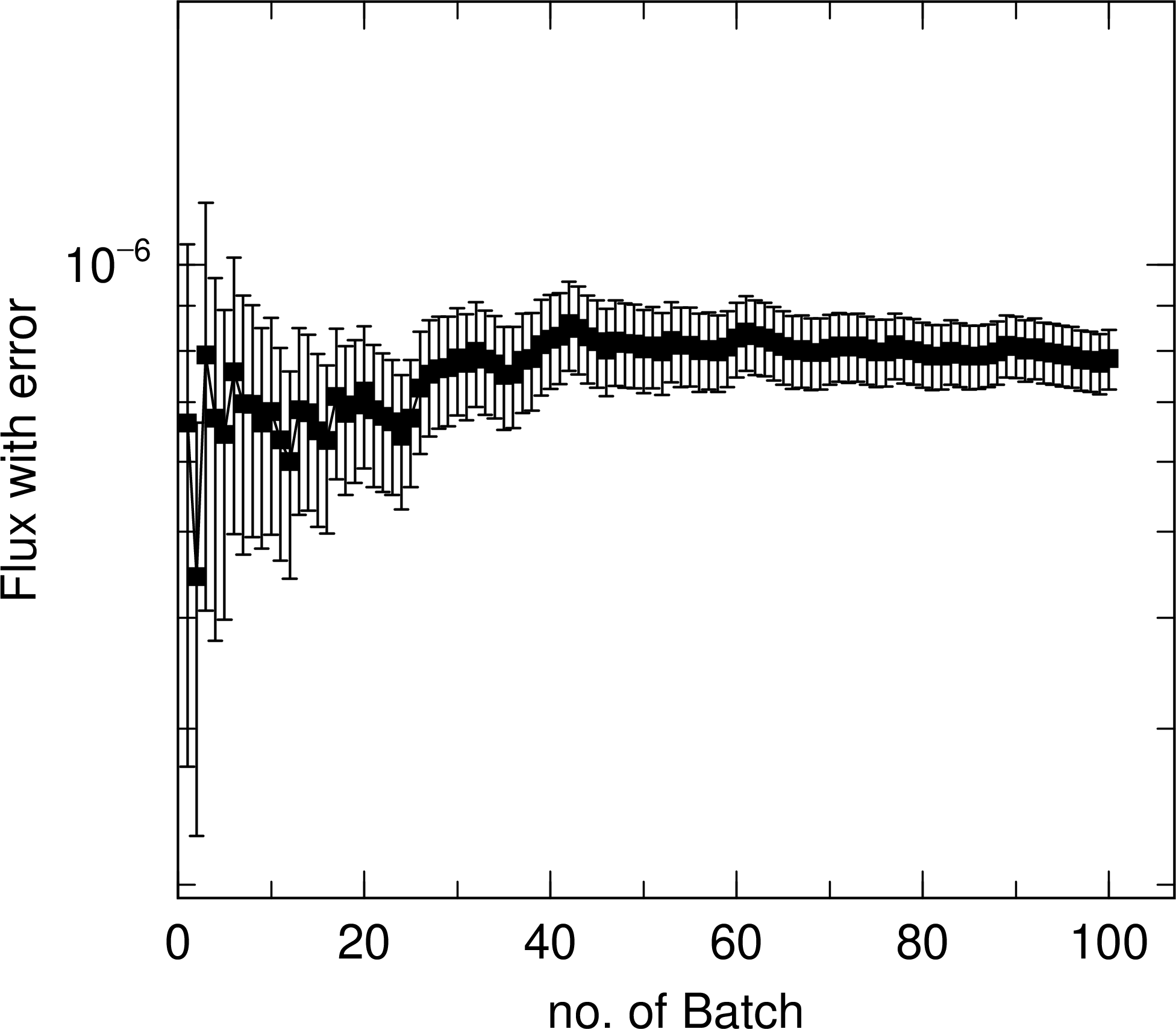
Fig. 6.10.1 Mean and statistical error as a function of the total number of histories (total number of batches).
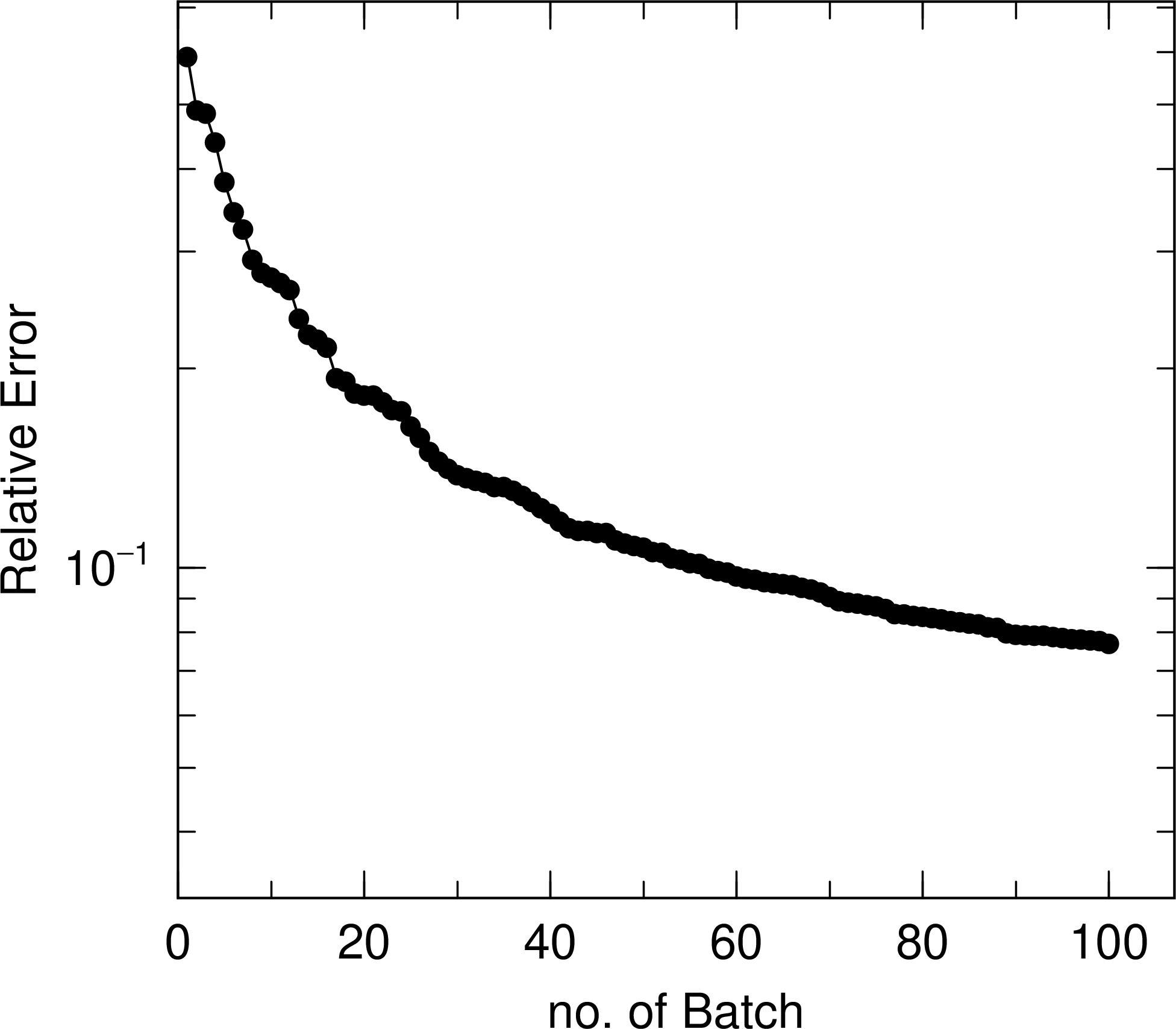
Fig. 6.10.2 Mean and statistical error as a function of the total number of histories (total number of batches).
6.10.2.2. B) Statistical check sheet and transition of the mean, statistical error, variance of the variance (VOV), and figure of merit (FOM) as a function of the total history number
In this case, VOV and FOM are added to the contents of A) and output as well as a statistical check sheet to check the reliability of these statistical indicators.
VOV is a statistical indicator of the degree of variance of statistical errors and is given as
Here, rewriting the mean \(\bar{x}\) in this equation by (6.10.1), VOV is given as follows:
PHITS calculates VOV using this expression. From the first term on the right-hand side, we can see that it has a dependency of \(1/N\) as well as the second term on the right-hand side, since the numerator is the sum of \(N\) and the denominator is the square of the sum of \(N\). Thus, when the statistic is sufficient, VOV will decrease by \(1/N\).
FOM is a statistical indicator of the degree of decrease in statistical error relative to computation time, using the ratio \(R\) of the standard error \(\sigma\) to the mean \(\bar{x}\) and the computation time \(T\) in minutes:
Since \(R\) is inversely proportional to the square root of \(N\), the value of FOM will be constant if \(T\) and the total number of histories \(N\) show a proportional relationship during a stable numerical calculation. Conversely, if the FOM changes significantly before or after a certain history, the proportional relationship between \(T\) and \(N\) has disappeared, and an anomaly such as a very long calculation time being required for that history can be confirmed.
In the case of B), PHITS outputs the statistical check sheet on the first page, and outputs the transition of the mean, statistical error, VOV, and FOM as a function of the total number of histories on the second, third, fourth, and fifth pages, respectively. Fig. 6.10.3 shows the statistical check sheet for the same calculation as in Fig. 6.10.1, where the column Quantity shows the type of statistical indicator and the column Output shows the type of value to be output. The Value column shows the value at the end of the batch, current value, and the value of dependence on the total number of histories, history dep. The pass column shows the result of determining whether or not the criteria are met. The method of evaluating the dependence on the total number of histories and the conditions for satisfying the criteria are explained in the next section. The results of Fig. 6.10.3 show that all but the criterion for the statistical error, less than 0.05, is satisfied, indicating that a stable calculation is being performed. However, since the statistical error is the most important indicator, it is desirable to increase the statistics to the extent that the criterion is met. Fig. 6.10.4 shows VOV and FOM as a function of the total number of histories. From the left panel, we can see that VOV shows a decreasing trend after 40 batches, decreasing at \(1/N\). On the other hand, from the results in the right panel, we can see how FOM converges to a constant value after 40 batches.
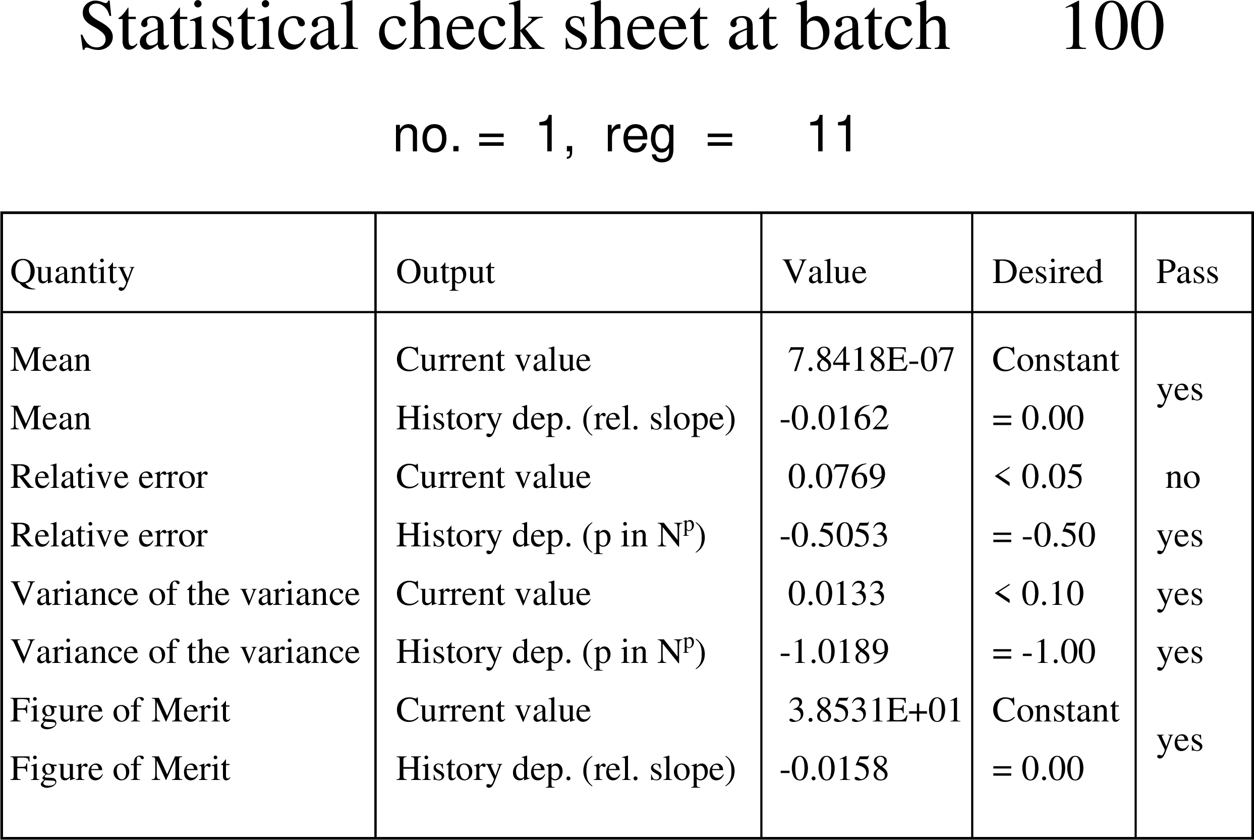
Fig. 6.10.3 Statistical check sheet at the end of 100 batches.
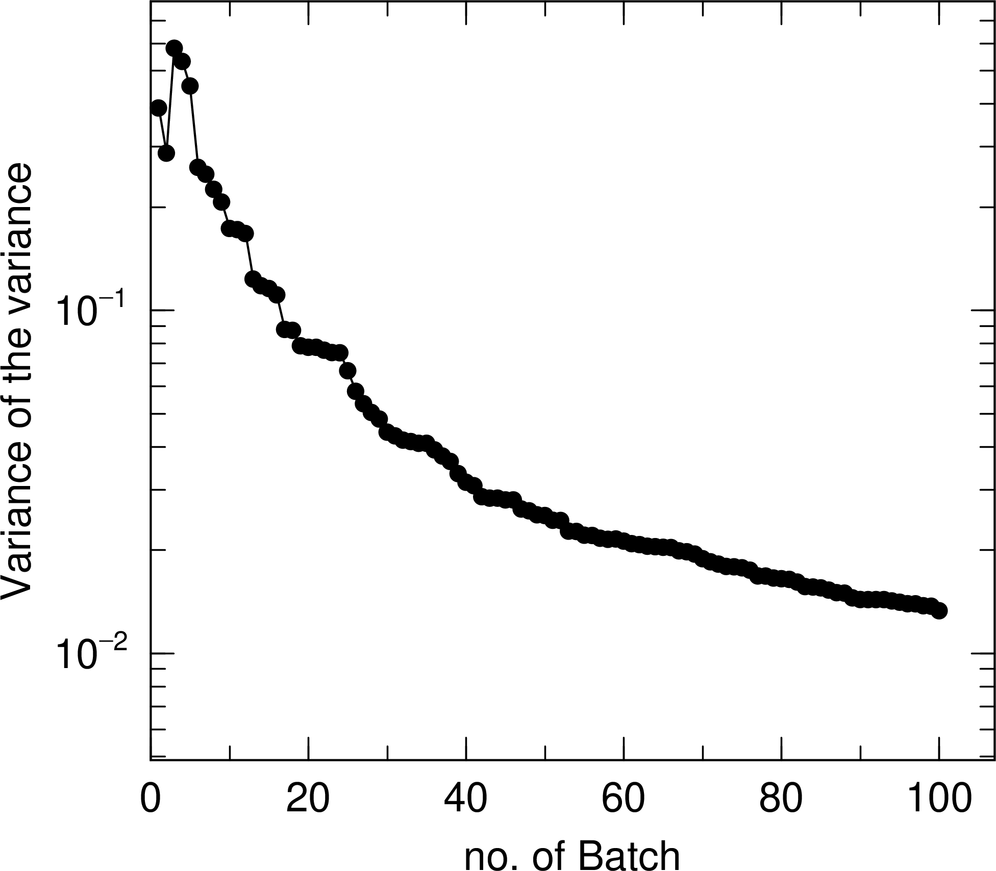
Fig. 6.10.4 Variance of variance (VOV) and figure of merit (FOM) as a function of the total number of histories (batches).
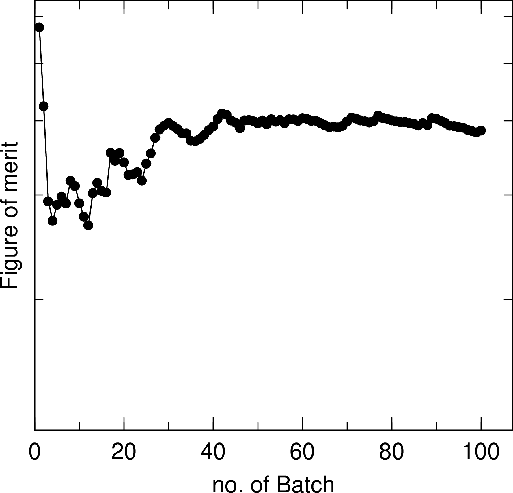
Fig. 6.10.5 Variance of variance (VOV) and figure of merit (FOM) as a function of the total number of histories (batches).
6.10.2.3. C) Statistical check sheet, transition of mean, statistical error, VOV, and FOM as a function of the total history number, and probability density function (PDF)
In this case, in addition to the contents of B), a PDF representing the distribution of the obtained tally results is output. Please note that there are two modes of calculation: a test calculation mode for confirming the range of output PDF, and a main calculation mode for explicitly specifying that range and obtaining the PDF. Basically, first confirm the range in the test calculation mode, and then perform the main calculation by specifying the lower limit prodenmn (D=1e-2) and upper limit prodenmx (D=1e+2) of the PDF range and the number of divisions nbproden (D=100).
For PDF calculations, the range of the PDF output \([x_{\rm min},x_{\rm max}]\) and the number of divisions \(n_{\rm pdf}\) on a logarithmic scale are determined, and when the tally result \(x_i\) for each history is obtained, which bin number it falls into is checked and the count number for that bin is increased. Finally, the output is normalized so that the distribution integrates to 1. Here, if the tally result is 0, it is not counted, so the peak position of the distribution and the mean \(\bar{x}\) may be shifted.
The test calculation mode works when none of the parameters prodenmn, prodenmx, and nbproden for PDF output are specified. In test calculation mode, calculations are started with initial values of \(x_{\rm min}=10^{-2}\), \(x_{\rm max}=10^2\), and \(n_{\rm pdf}=100\), and if tally results are outside of the range \([x_{\rm min},x_{\rm max}]\), the upper or lower limit of the range is changed according to the size of the result. For example, if a tally result of \(10^3\) is obtained, the upper limit is 10 times the tally result and \(x_{\rm max}=10^4\). On the other hand, if a smaller tally result is obtained, then 1/10 of that value is used as \(x_{\rm min}\). In this way, by confirming the distribution of the final output PDF, we can see the range that the tally result can take. Note that if the tally result differs from the initial value \(x_{\rm min}=10^{-2}, x_{\rm max}=10^2\) by several tens of digits, the range of the horizontal axis of the output PDF will expand by that number of digits. In such a case, please adjust manually while specifying the output range in the main calculation mode shown below. Note that in the test calculation mode, the stored PDF data is reset each time the range changes due to adjustment, so results for a different number of histories are output than for other statistical indicators. Parallel computation by MPI or OpenMP cannot be used for the test calculation.
Next, the main calculation mode operates if any one of prodenmn, prodenmx, and nbproden is specified. Parameters not explicitly specified will be set to their respective default values. In this calculation mode, the range of tally results to be stored does not change during the PHITS running, and a PDF of the tally results is output. However, if a tally result is larger than the upper limit of the set range, a warning message is output. The message output stops after about 5 times, when parallel calculation is not used, but if this message appears, stop the calculation once and increase the upper limit prodenmx and run the main calculation mode again. In this calculation mode, parallel calculation by MPI or OpenMP can be used.
In the case of C), pages 1 through 5 are the same as in B). In addition, the PDF at the end of the batch is output on page 6. Fig. 6.10.6 shows the PDF for the same calculation as in Fig. 6.10.1. Although the statistics are not sufficient to determine a normal distribution, we can see that the distribution has a peak around \(10^{-3}\) and the tally results in values within the range of approximately \(10^{-4}\) to \(10^{-2}\). The mean of this tally result is about \(10^{-6}\), which is about 3 orders of magnitude different from the peaked value of \(10^{-3}\), indicating that the percentage of non-zero tally results is about 1/1000.
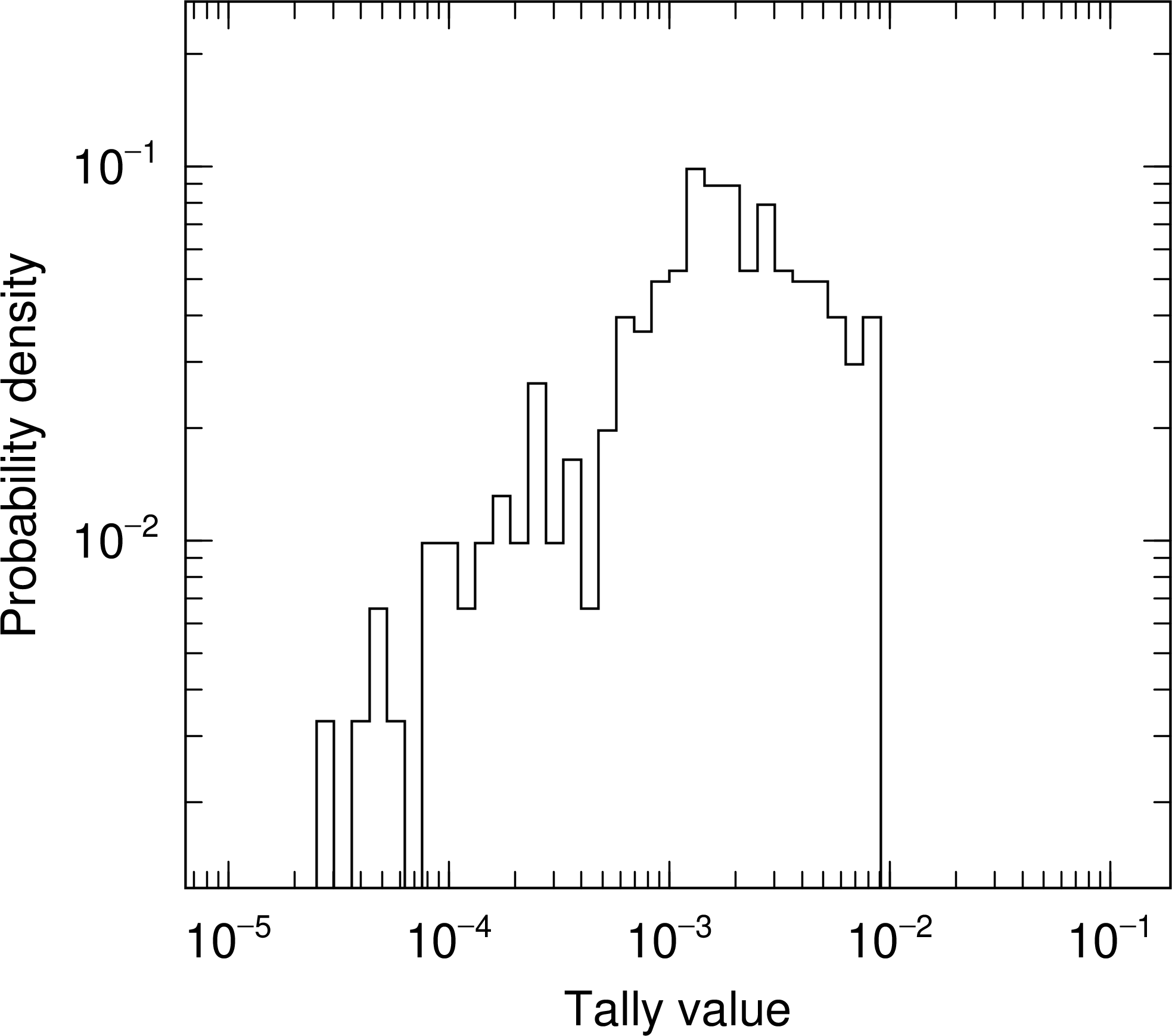
Fig. 6.10.6 Probability density function (PDF) of tally results.
The PDF is an indicator that allows direct confirmation of the specific numerical values of the tally results, making it easier to detect anomalies, for example, having values in areas outside the distribution, especially toward larger values. Note that to confirm a clean distribution structure, a larger number of histories is required than for other statistical indicators. For this reason, PDFs are not considered in the statistical check sheet.
6.10.3. Statistical check sheet
This check sheet outputs the current value at the end of the batch for the mean, statistical error, variance of the variance (VOV), and figure of merit (FOM), and their dependence on the total number of histories, history dep., and a total of six checkpoints are judged yes or no by comparing them to criterion values.
The dependence on the number of histories is evaluated from the results of the second half of all histories. For example, when calculations of 100 batches are finished, the values from batch 51 to 100 are used. Since the mean and FOM are independent of the total number of histories, that is, converge to a constant value, a function \(f(N_{\rm batch})=aN_{\rm batch}+b\), where \(N_{\rm batch}\) is the total number of batches, is assumed and fitted by the least squares method, and its coefficient \(a\) is close to 0 or not. Specifically, if the absolute value of this coefficient normalized by the value at the last batch is less than 0.05, it is judged as yes. If it is greater than 0.05, it is judged as no. The statistical error is proportional to the inverse of the square root of the total number of histories, so the function \(f(N_{\rm batch})=b\exp(aN_{\rm batch})\) is assumed and fitted by the least squares method, and judged if the coefficient \(a\) is close to \(-0.5\). Specifically, if it is in the range of \(-0.9475\) to \(-0.525\), it is assumed to be yes. For VOV, since it is inversely proportional to the total number of histories, the least squares method is performed assuming a function similar to that for statistical errors, and it is determined if the coefficient \(a\) is close to \(1.0\) or not. Specifically, if it is in the range of \(-0.95\) to \(-1.05\), it is assumed to be yes.
Please note that the criterion values used to determine PASS in this checklist are not absolutely reliable. Depending on the calculation conditions and the desired accuracy of the calculation, the criterion values for judging the reliability of the calculation results may change. Just because all six are yes does not mean that the results are always reliable. On the other hand, even if an item is no, you may be able to determine that there is no problem by checking the transition of that statistical indicator as the total number of histories increases.