5.6. [ Cell ] section
5.6.1. Formats
In the [cell] section, cells can be defined in terms of surfaces described in the [surface] section. A cell should be set as a closed space, and a virtual space for particle transport calculation can be generated by combining defined cells. In PHITS, an outer void must be explicitly defined as a cell.
Only $ and c (with a following half-width space) can be used as comment marks in this section; in particular, # cannot be used as a comment mark because this character is used for the cell definition. To use continuation lines, it suffices to place at least five blanks at the line head instead of using the line sequential mark at the end of the line.
The [cell] section is defined in this data order: cell number, material number, material density, cell definition, and cell parameter as keyword style. These are explained in Table 5.6.1. The format is shown below.
[ Cell ]
  cell number  mat. number  mat. density  cell def.  cell parameter
In the LIKE n BUT format, the cell parameter format and repeated structures with lattices can be used: see Section 5.6.5 for some examples showing how to use this format. The cell parameters are listed and explained in Table 5.6.2.
item |
explanation |
|---|---|
cell number |
Any number from 1 to 999,999 can be used. |
material number |
Set 0 for void, |
material density |
Gives the density of the material in the cell. If the value is 0, the density defined in the [material] section is used as is. If the value is positive, it is treated as a particle density [\(10^{24}\) atoms/cm\(^3\)]; if negative, it is treated as a mass density [g/cm\(^3\)]. When the value is not 0, the density specified here is used in the transport calculation, while the composition ratio is determined on the basis of the density defined in the [material] section. Therefore, materials with the same composition but different densities can be defined. The parameter matadd can be used to assign different material numbers in such cases. If the cell is void, namely when the material number is 0 or -1, this item is omitted. |
cell definition |
Cell geometry is defined by both surface numbers in the [surface] section and the Boolean operators, blank space (AND), : (OR), and # (NOT). Parentheses ( and ) can also be used. See Section 5.6.2 for details. |
LIKE n BUT |
A cell using this format is the same as an |
cell parameter |
The format is keyword=value. As a keyword, VOL (volume), TMP (temperature), TRCL (transform), U (universe), LAT (lattice), or FILL can be used. In the LIKE n BUT format, MAT (material) and RHO (density) can be used as well. |
When defining cells with the same material number but different densities, the cells assume material numbers that differ from that of the first cell.
In operation of the cell definition, blank space has a higher priority than :.
item |
explanation |
|---|---|
VOL |
Volume [cm\(^3\)] of the cell is given. |
TMP |
Temperature [MeV] of the material in the cell is given. |
TRCL |
Coordinate transform for position of the cell is performed using the defined coordinate transform number in the [transform] section or the transform format. |
U |
Universe number; using this, the number of the universe including the cell is defined. Any number value can be used from 1 to 999,999. See Section 5.6.3 for details. |
LAT |
Lattice number. Setting LAT=1 or LAT=2 defines a quadratic or hexangular prism, respectively: see Section 5.6.4 for details. |
FILL |
Set universe numbers to fill the cell with the universe. |
MAT |
This is used with the LIKE n BUT MAT=m format. Using
MAT, a cell can be duplicated except with its material number
changed to |
RHO |
This is used with the LIKE n BUT RHO=x format. Using
RHO, a cell can be duplicated except with its density changed
to |
5.6.2. Description of cell definition
Cells are defined by treating regions divided by surfaces defined in the [surface] section. When giving a cell definition, in some cases the concept of surface sense must be used to create a distinction between two regions divided by the surface corresponding to an equation, \(f(x,y,z)=0\); in other cases, the Boolean operators, blank space (AND), : (OR), and # (NOT), must be used to treat the regions.
Surface sense defines one region including a point \((x_0,y_0,z_0)\) by treating \(f(x_0,y_0,z_0)>0\) in a positive sense, and the region \(f(x_0,y_0,z_0)<0\) in a negative sense. To define a region in the positive sense, a positive surface number is written in the cell definition space; conversely, a negative surface number is used in the definition to denote a negative sense. An example of the definition of sense is shown below.
     1:   [ Cell ]
     2:     1   0  -10
     3:     2  -1   10
     4:   [ Surface ]
     5:     10  SZ  3  5
The tenth surface represents a sphere with a radius of 5 cm. Because the inside of this sphere is in the negative sense, the first cell is defined using a negative number -10. The outer void is explicitly defined as the second cell. This example produces the virtual space shown in Fig. 5.6.1.
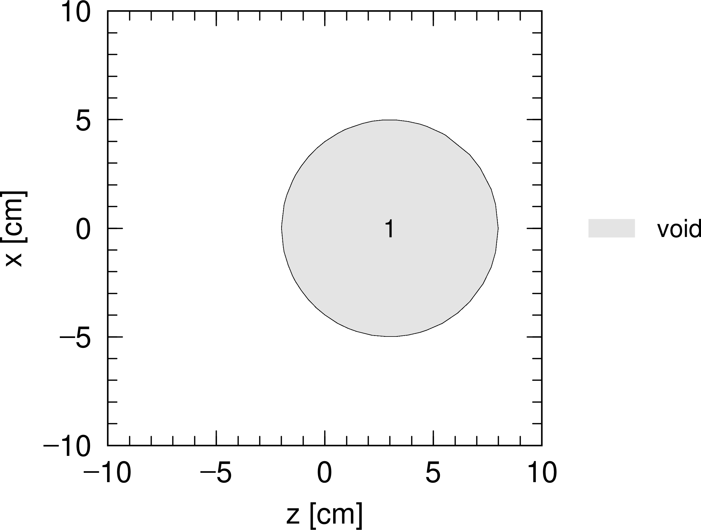
Fig. 5.6.1 Result of [cell] section example (1).
In some cases, the treatment of a region in the cell definition involves the use of Boolean operators. The symbols blank space, :, and # denote the intersection (AND), union (OR), and complement (NOT) operators, respectively. When using #all, it excludes all cells except for those defined as the outer void or in other universes, making it convenient for defining the entire phase space. For the preprocessing function that helps expand #all, see Section 5.7. Parentheses, e.g. ( and ), can be used to combine some regions. The second example in this section uses blank space and #.
     1:   [ Cell ]
     2:     1   0  11  -12  13  -14  15  -16
     3:     2  -1  #1
     4:   [ Surface ]
     5:     11  PX  -6
     6:     12  PX   6
     7:     13  PY  -6
     8:     14  PY   6
     9:     15  PZ  -6
     10:     16  PZ   6
In the cell definition in the second line, the three numbers without minus signs correspond to the positive sense regions of the eleventh, thirteenth, an fifteenth surfaces, while those with minus signs correspond to the negative sense regions of the twelfth, fourteenth, and sixteenth surfaces. A region surrounded by these surfaces is defined with blank space as the first cell, which is the interior of a 12-cm cube. The outside of the cube is defined by the complement operator # as the outer void. Fig. 5.6.2 shows the result of this example.
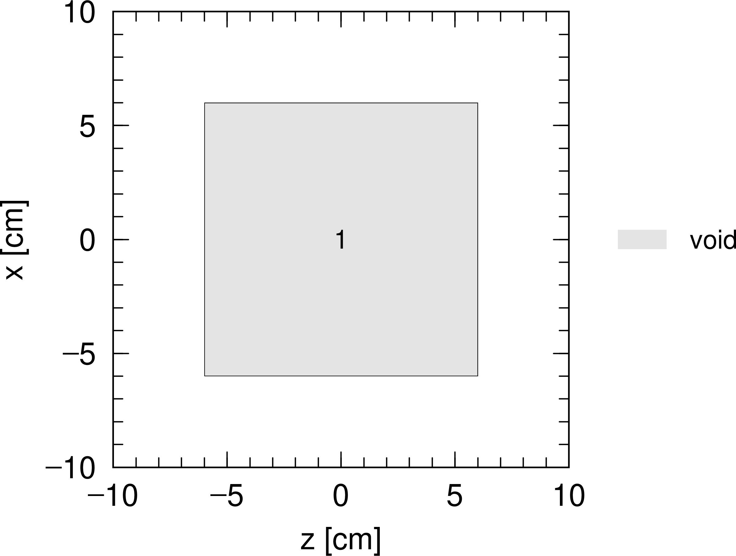
Fig. 5.6.2 Result of [cell] section example (2).
The next example uses: and parentheses to combine the sphere in the first example and the cube in the second example.
     1:   [ Cell ]
     2:     1   0  -10 : (11  -12  13  -14  15  -16)
     3:     2  -1  #1
     4:   [ Surface ]
     5:     10  SZ   3  5
     6:     11  PX  -6
     7:     12  PX   6
     8:     13  PY  -6
     9:     14  PY   6
    10:     15  PZ  -6
    11:     16  PZ   6
The numbers surrounded by the parentheses in the second line correspond to the region of the first cell in example (2). In this example, a region combining the inside of the cube with the inside of the sphere in example (1) is defined using the union operator: as the first cell. The result is shown in Fig. 5.6.3.
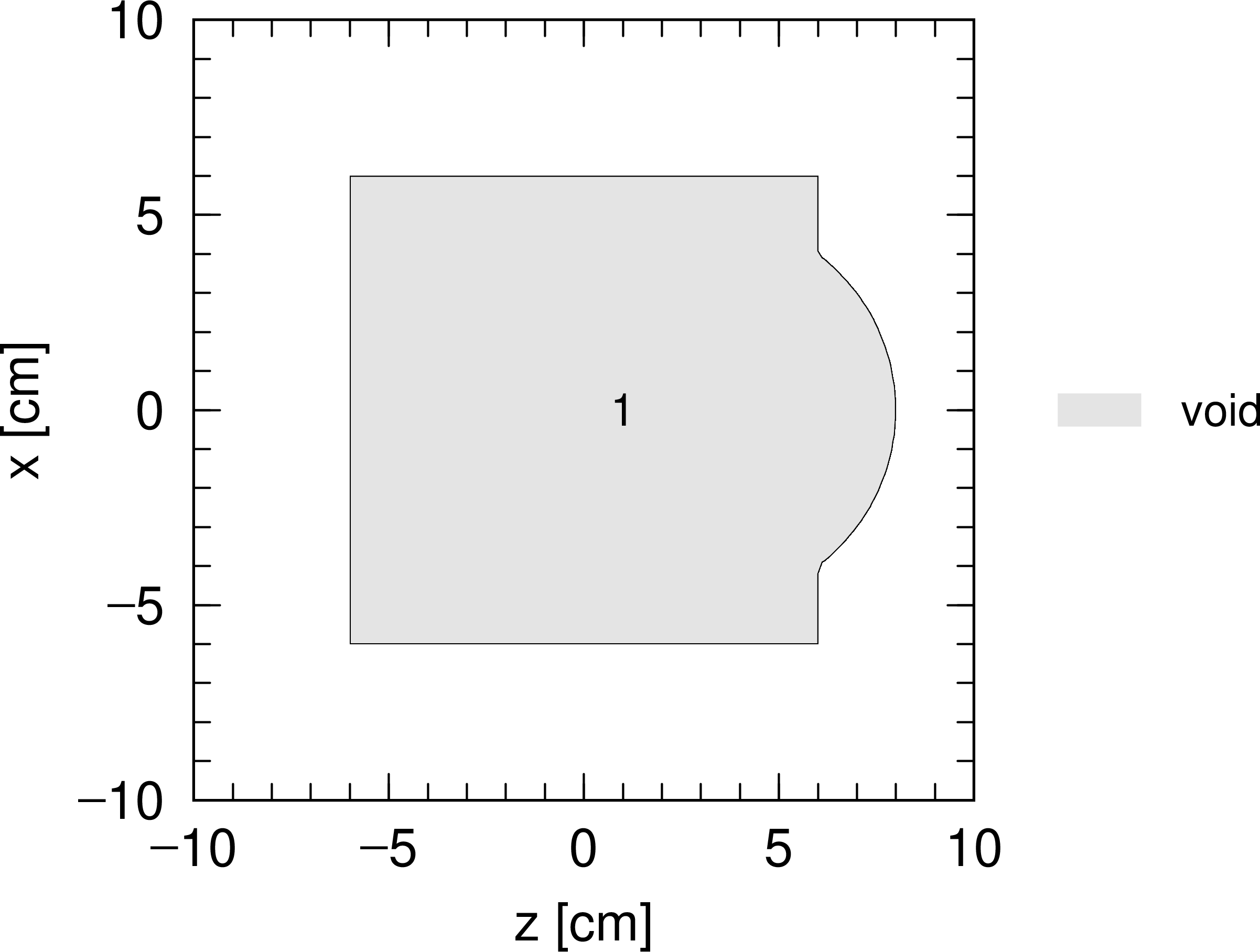
Fig. 5.6.3 Result of [cell] section example (3).
The next example shows the division of a cube into two regions by a spherical surface.
     1:   [ Material ]
     2:     mat[1]  1H 2  16O 1
     3:   [ Cell ]
     4:     1   0       -10
     5:     2   1  -1.0   10 (11  -12  13  -14  15  -16)
     6:     3  -1        #1 #2
     7:   [ Surface ]
     8:     10  SZ   3  5
     9:     11  PX  -6
    10:     12  PX   6
    11:     13  PY  -6
    12:     14  PY   6
    13:     15  PZ  -6
    14:     16  PZ   6
This [surface] section is the same as in example (3). In the fifth line, the second cell is defined with blank space as an overlap region between the outside of the sphere, which is the tenth surface, and the inside of the cube defined by the parentheses. The cell is filled with water as defined in the [material] section and the result is shown in Fig. 5.6.4. The interior of the sphere is the first cell, which is filled with void.
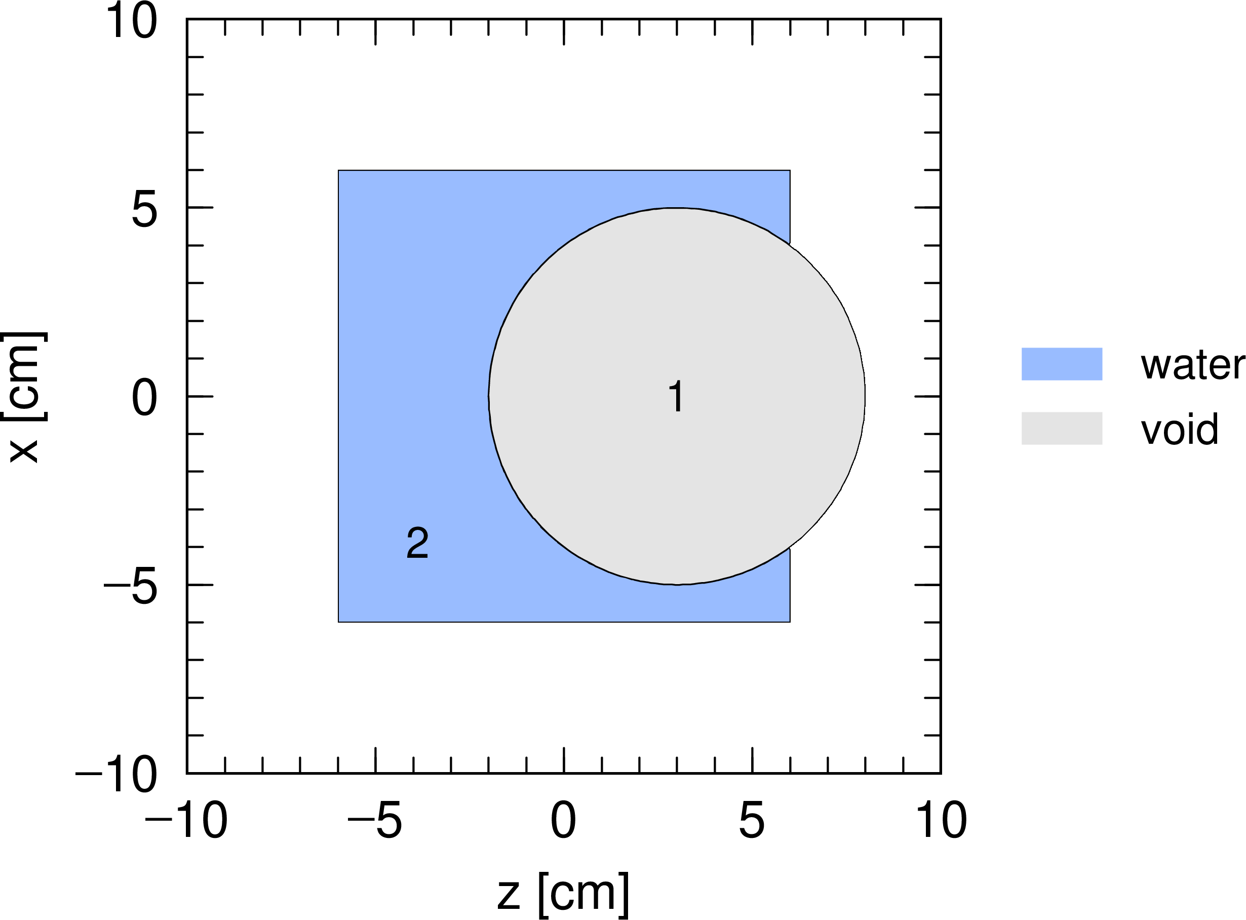
Fig. 5.6.4 Result of [cell] section example (4). The first and second cells are filled with void and water, respectively.
Even empty areas (such as vacuum or air) must be defined in a way that avoids overlapping definitions with other regions. In such cases, use of #all command, which excludes all other regions except for those for outer void and in other universe (see next section), is convenient. For the preprocessing function that automatically expands cells containing #all, see Section 5.7. Note that only one #all can be defined per input file. If you also want to exclude the outer-void region from a region defined using #all, directly exclude the cell number defined as the outer void with #. For example, if the outer void is defined as cell 9, you can write #all #9. In this case, a warning message is output, but it can be safely ignored if you intentionally exclude the outer-void region in this way.
5.6.3. Universe frame
In PHITS, the cell parameter U can be used to define a region of the main space used for particle transport calculation that can be translated to a corresponding region in any universe. This function is very useful for setting the repeated structures introduced in Section 5.6.5.
An example using three spaces (one main space and two universes), shown below, is explained below. The main space comprises two rectangular solids. One universe includes a cylinder filled with water, while the other has an iron cylinder surrounded by water. The first cell is filled with a region of universe 1, while the second cell is filled with a region of universe 2.
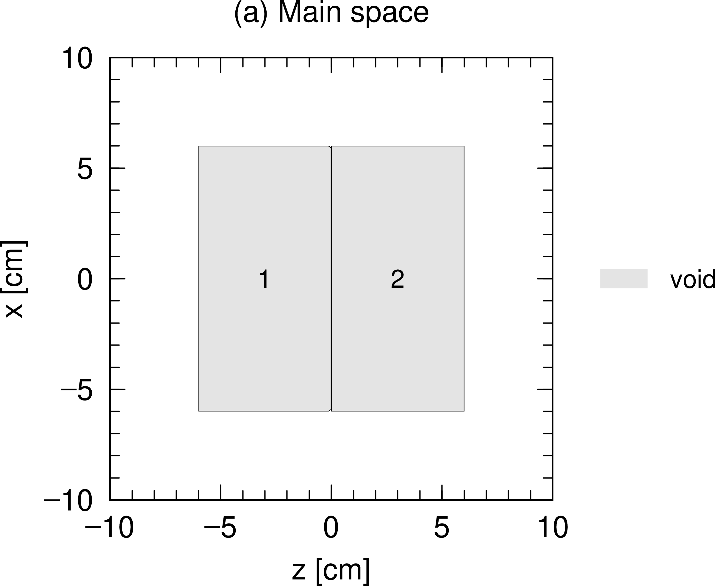
Fig. 5.6.5 Two rectangular solids.
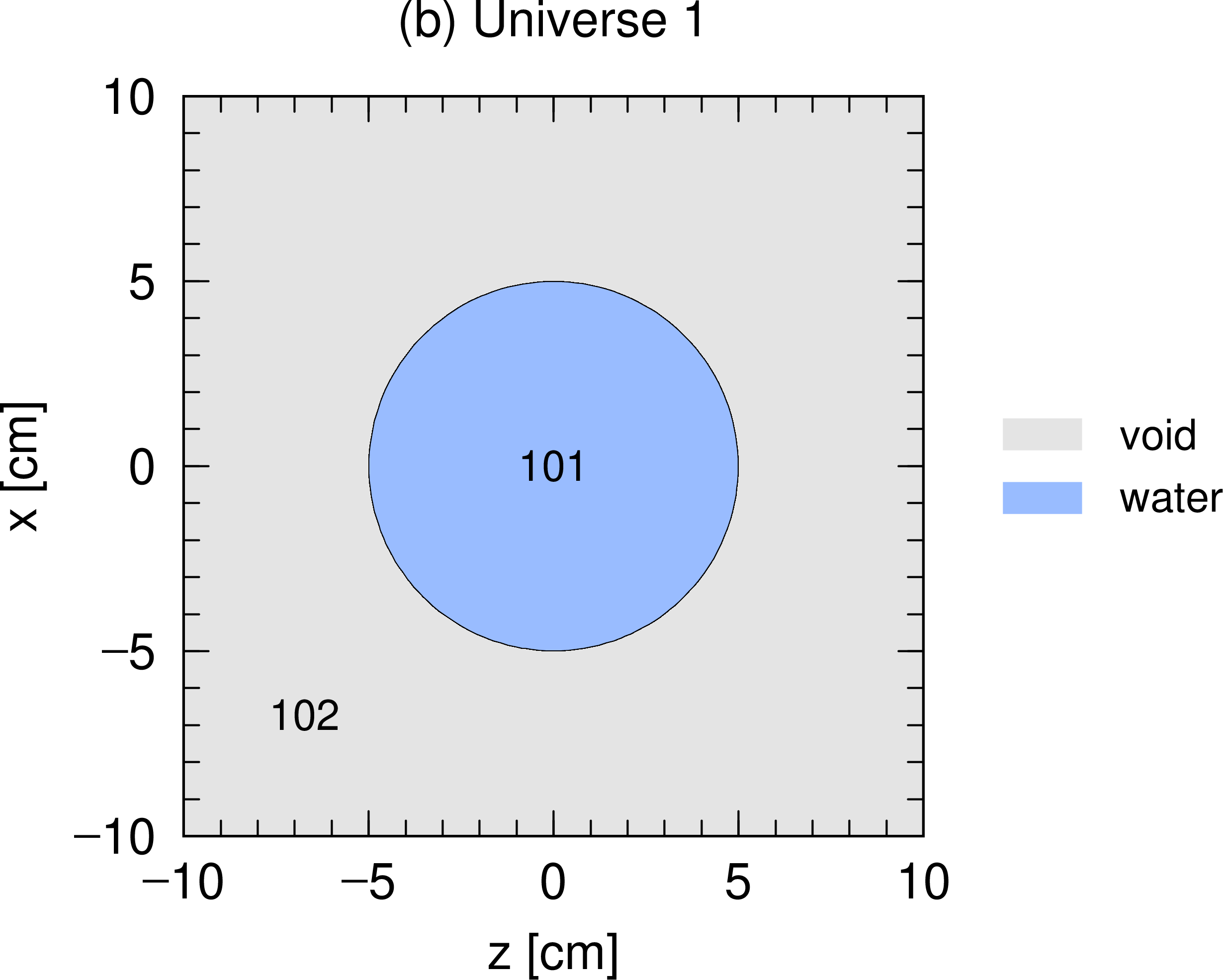
Fig. 5.6.6 Cylinder filled with water.
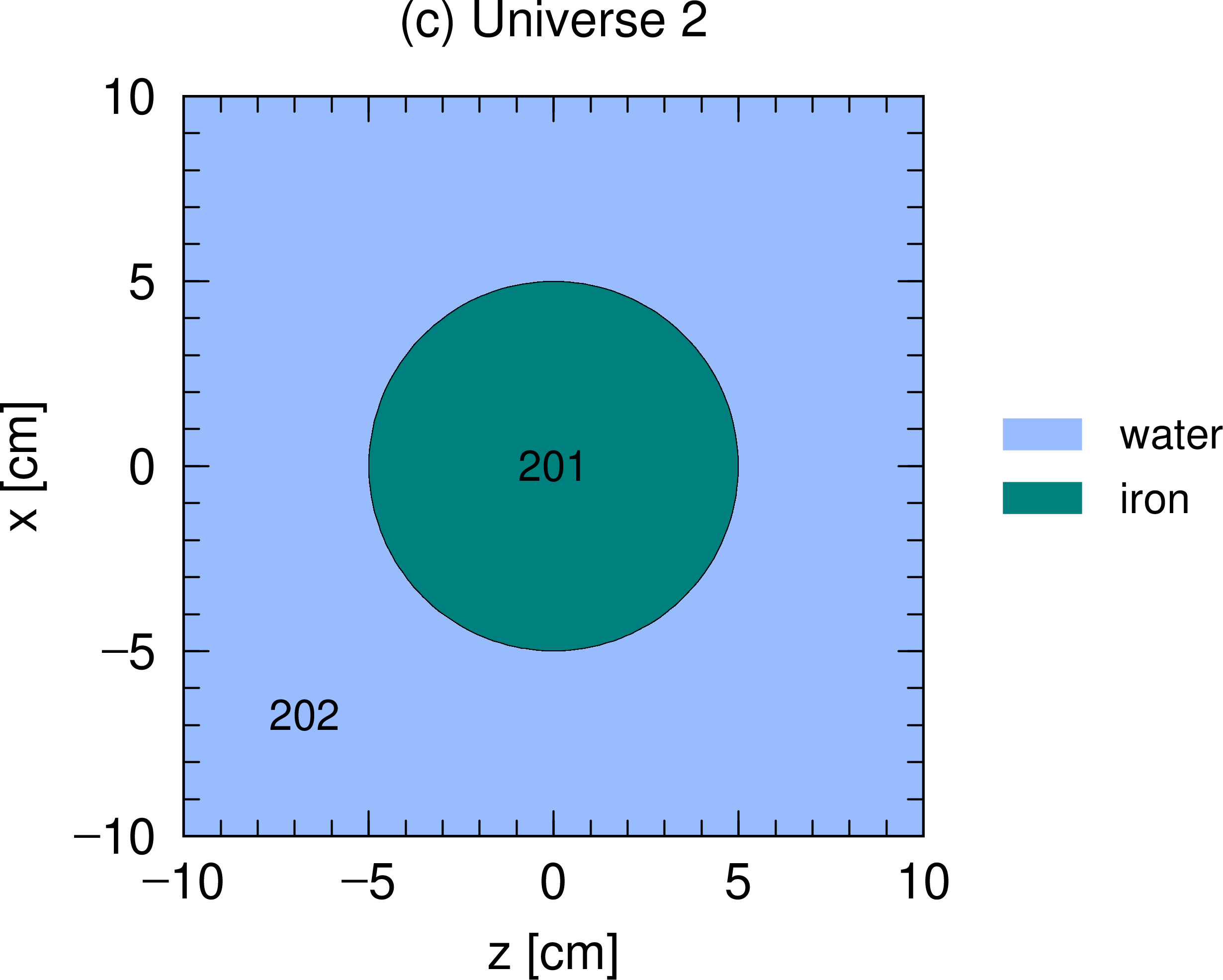
Fig. 5.6.7 Iron cylinder in water.
     1:   [ Material ]
     2:     mat[1]  1H 2  16O 1
     3:     mat[2]  Fe 1
     4:   [ Cell ]
     5:       1  0        11  -12  13  -14  15  -17  FILL=1
     6:       2  0        11  -12  13  -14  17  -16  FILL=2
     7:     101  1  -1.0  -10  13  -14  U=1
     8:     102  0       #101  U=1
     9:     201  2 -10.0  -10  13  -14  U=2
    10:     202  1  -1.0  #201  U=2
    11:       9 -1       #1 #2
    12:   [ Surface ]
    13:     10  CY   5
    14:     11  PX  -6
    15:     12  PX   6
    16:     13  PY  -6
    17:     14  PY   6
    18:     15  PZ  -6
    19:     16  PZ   6
    20:     17  PZ   0
Universes 1 and 2 are defined in the seventh and eighth lines and in the ninth and tenth lines, respectively, using cell parameter U. These universes have similar structures in which a cylinder is placed at the origin of the coordinate space, but their components inside and outside the cylinder differ, as shown in the figures above. In the fifth and sixth lines, the first and second cells are defined respectively as regions filled with the corresponding part of each universe using the cell parameter FILL. The result of this example is shown in Fig. 5.6.8, in which it can be seen that the first cell comprises the 101st and 102nd cells in universe 1, while the second cell comprises the 201st and 202nd cells in universe 2.
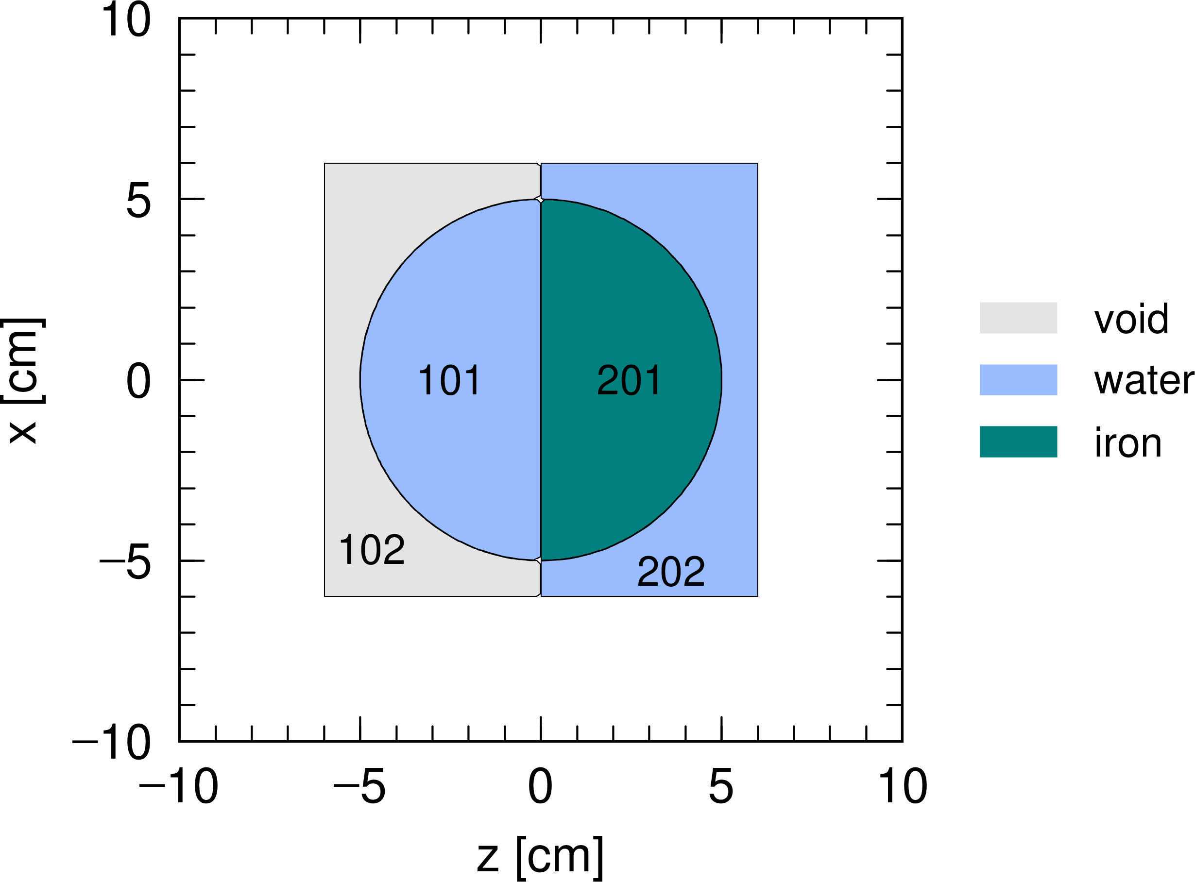
Fig. 5.6.8 Result of [cell] section example (5).
It is not possible to use an undefined region from one of the universes. If the 102nd cell is not defined in the eighth line as a void region, the first cell cannot be filled with universe 1. Note also that all universes have the same coordinate system definition, with the position of the origin, directions of \(x\), \(y\), and \(z\)-axes, and scale of the space in any universe agreeing with those in any other universe. If a different value of PX is in the fourteenth and fifteenth lines, the cube will not include some of the cylinder, as shown in Fig. 5.6.9.
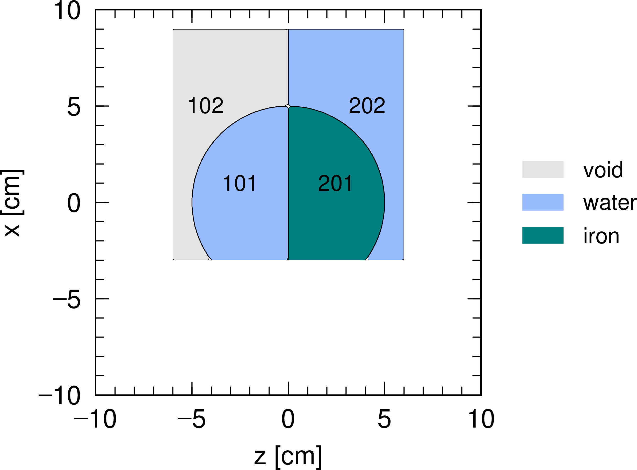
Fig. 5.6.9 Result of [cell] section example (5) with the region shifted in the \(x\)-direction.
5.6.4. Lattice definition
The cell parameter LAT (lattice parameter) is very useful for making repeated structures. In this section, the definition of a unit lattice structure and its simple use are explained using some examples: see Section 5.6.5 for a more practical description.
The quadratic and hexangular prisms shown in Fig. 5.6.10 can be used as a unit structure by setting LAT=1 or LAT=2, respectively. A universe can be constructed using repeated structure of such a lattice, and any region can be filled using this universe. Note that each unit must also be filled with another universe define with any material or void. The numbering of each unit component in Fig. 5.6.10 corresponds to the surface number order written in the cell definition; the lattice coordinate system, which will be explained below, depends on this order.
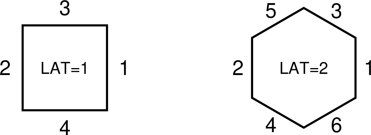
Fig. 5.6.10 Unit structure of lattice.
An example using a quadratic prism (LAT=1) is shown below.
     1:   [ Material ]
     2:     mat[1]  1H 2  16O 1
     3:   [ Cell ]
     4:       1   0        11  -12   13  -14   15  -16  FILL=1
     5:     101   0       -26   25  -24   23  -22   21  LAT=1  U=1  FILL=2
     6:     201   1  -1.0  -90  U=2
     7:       2  -1       #1
     8:   [ Surface ]
     9:     11  PX  -6
    10:     12  PX   6
    11:     13  PY  -6
    12:     14  PY   6
    13:     15  PZ  -6
    14:     16  PZ   6
    15:     21  PX  -2
    16:     22  PX   2
    17:     23  PY  -2
    18:     24  PY   2
    19:     25  PZ  -2
    20:     26  PZ   2
    21:     90  BOX  -10 -10 -10  20 0 0  0 20 0  0 0 20
In the fifth line, a unit cell with LAT=1 is defined using four surface numbers. Setting U=1 defines as the repeated structures of this unit, which is filled with universe 2 defined in the sixth line. Because the cross section of the unit in the \(x\)-\(z\) plane is a square four cm per side, the first cell defined in the fourth line as a 12 cm cube has nine blocks, as shown in Fig. 5.6.11. Note that the unit has an infinite length in the \(y\) direction of universe 1 because only four surfaces are defined. To define a finite-length prism, -24 23 must be added to the cell definition in the fifth line.
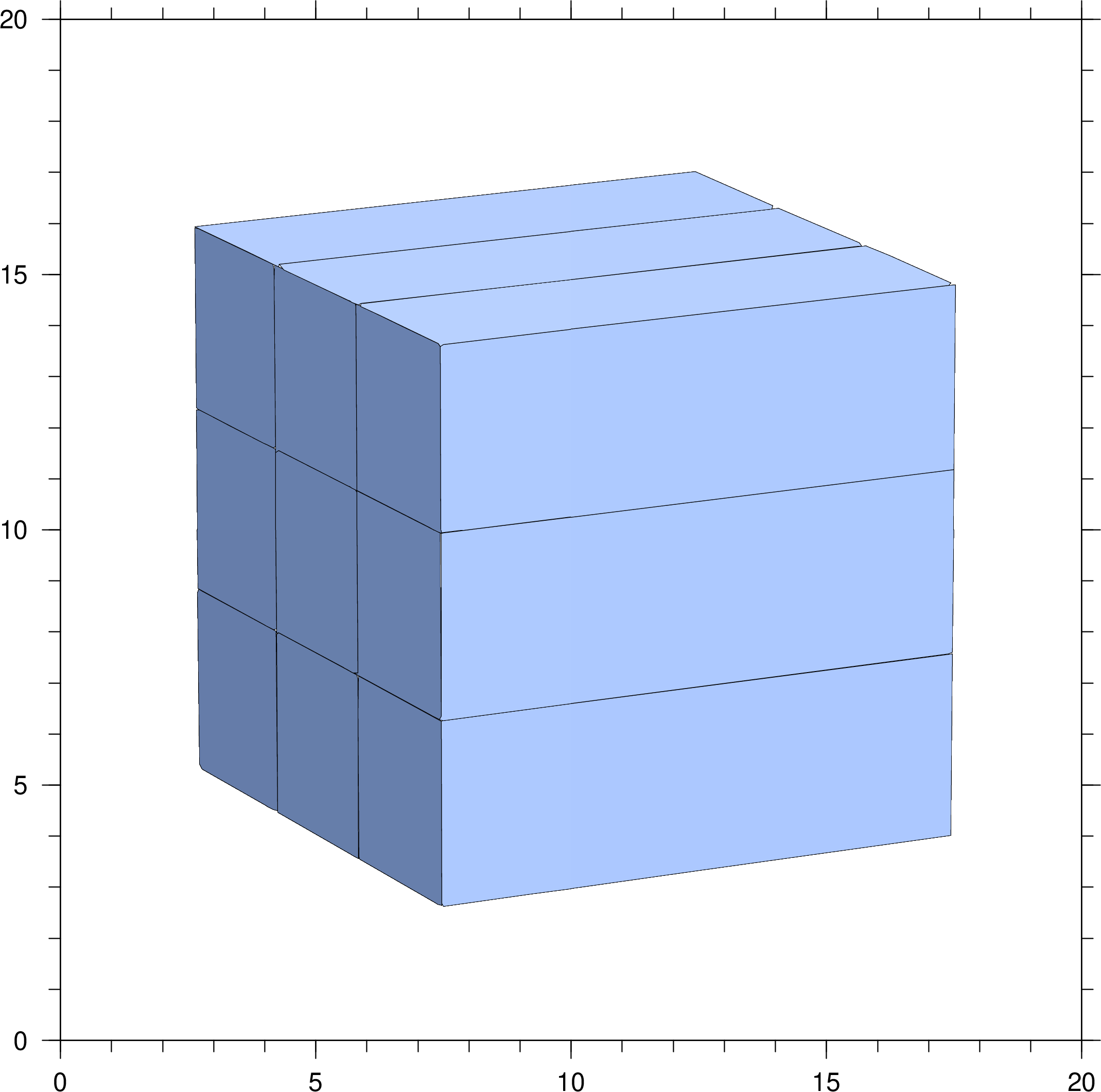
Fig. 5.6.11 Result of [cell] section example (6) in 3D images.
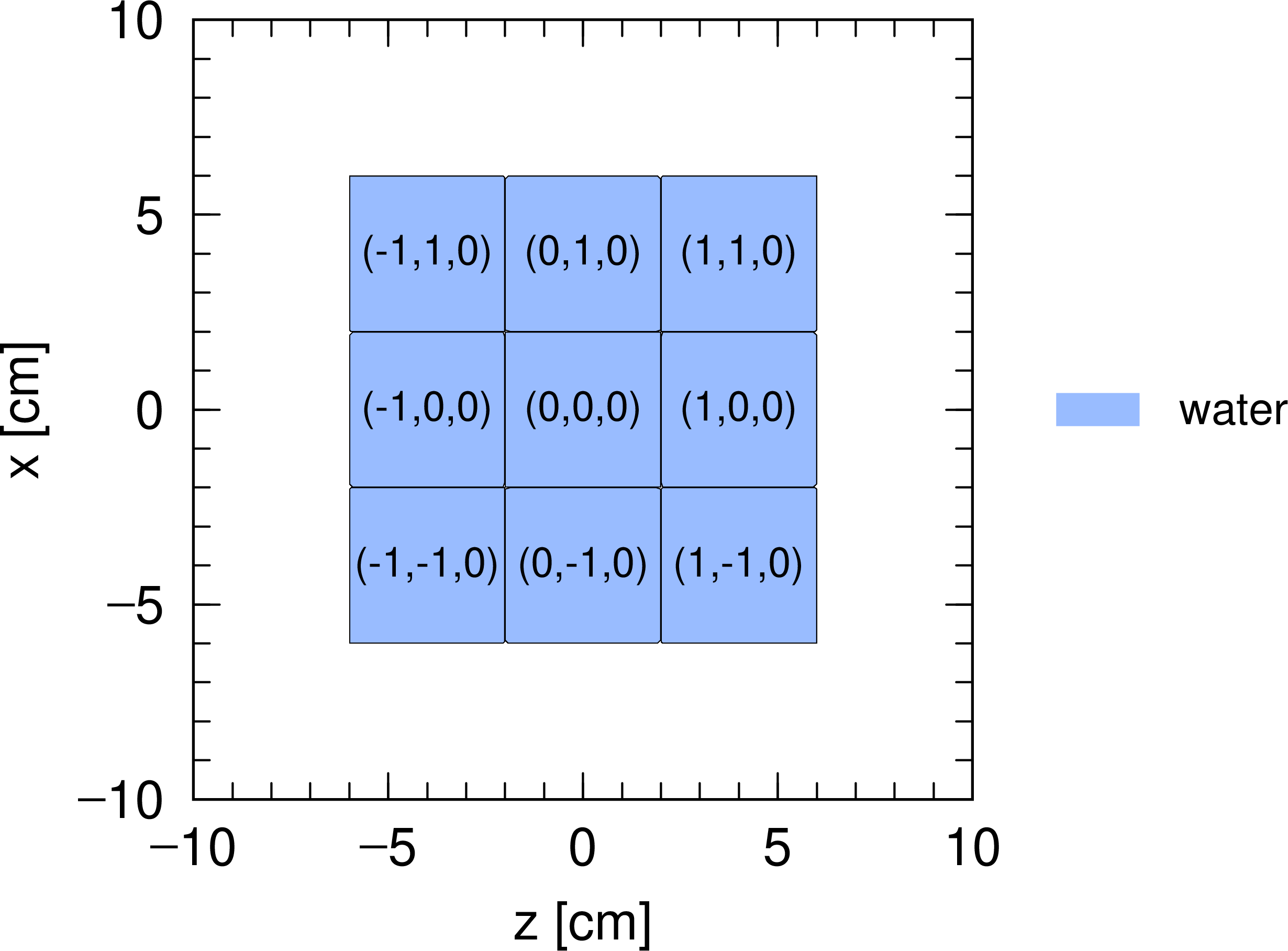
Fig. 5.6.12 Result of [cell] section example (6) in 2D images.
To distinguish cells in the repeated structure, each cell is placed at the lattice coordinate \((i,j,k)\), as shown in Fig. 5.6.12.
Note that the ordering of this coordinate notation corresponds to the general coordinate ordering \((x,y,z)\) and is defined by the order of surface numbers written in the cell definition.
To specify any cell using mesh=reg in a tally section, the lattice and universe styles (201 < 101[-1 0 0]) can be used, where the lattice coordinate is represented by [i j k]: see Sec. Volume definition for more information on this format.
The lattice coordinates can be viewed using the [t-gshow] tally with output=7 or 8.
The following example involves a hexangular prism (LAT=2).
     1:   [ Material ]
     2:     mat[1]  1H 2  16O 1
     3:   [ Cell ]
     4:       1   0        11 -12  13 -14  15 -16  FILL=1
     5:     101   0       -31  32 -33  34 -35  36 -24  23  LAT=2  U=1  FILL=2
     6:     201   1  -1.0  -90  U=2
     7:       2  -1       #1
     8:   [ Surface ]
     9:     11  PX  -6
    10:     12  PX   6
    11:     13  PY  -6
    12:     14  PY   6
    13:     15  PZ  -6
    14:     16  PZ   6
    15:     23  PY  -2
    16:     24  PY   2
    17:     set: c1[2]
    18:     31  PZ  [ c1*cos(pi/6)]
    19:     32  PZ  [-c1*cos(pi/6)]
    20:     33  P   1  0  [ 1/tan(pi/3)]  [ c1]
    21:     34  P   1  0  [ 1/tan(pi/3)]  [-c1]
    22:     35  P   1  0  [-1/tan(pi/3)]  [ c1]
    23:     36  P   1  0  [-1/tan(pi/3)]  [-c1]
    24:     90  BOX  -10 -10 -10  20 0 0  0 20 0  0 0 20
A hexagon with LAT=2 is defined in the fifth line using the six surfaces defined in the seventeenth through twenty third lines.
The hexagonal prism is restricted in the \(y\)-direction by -24 23 in the cell definition and is filled with universe 2, i.e. water, as specified in the sixth line.
The first cell has the repeated structure defined in universe 1.
Fig. 5.6.13 shows the result of this example.
It can be seen that some prisms near the edges of the first cell, which is defined as a 12 cm cube, are only partly used.
The directions of the lattice coordinate shown in Fig. 5.6.14 depend on the order of the surface number written in the cell definition.
To specify a cell using mesh=reg in a tally section, the lattice and universe styles (201 < 101[-2 0 0]), where the lattice coordinate is represented by [i j k], can be used: see Sec. Volume definition for more information on this format.
The lattice coordinates can be shown using the [t-gshow] tally with output=7 or 8.
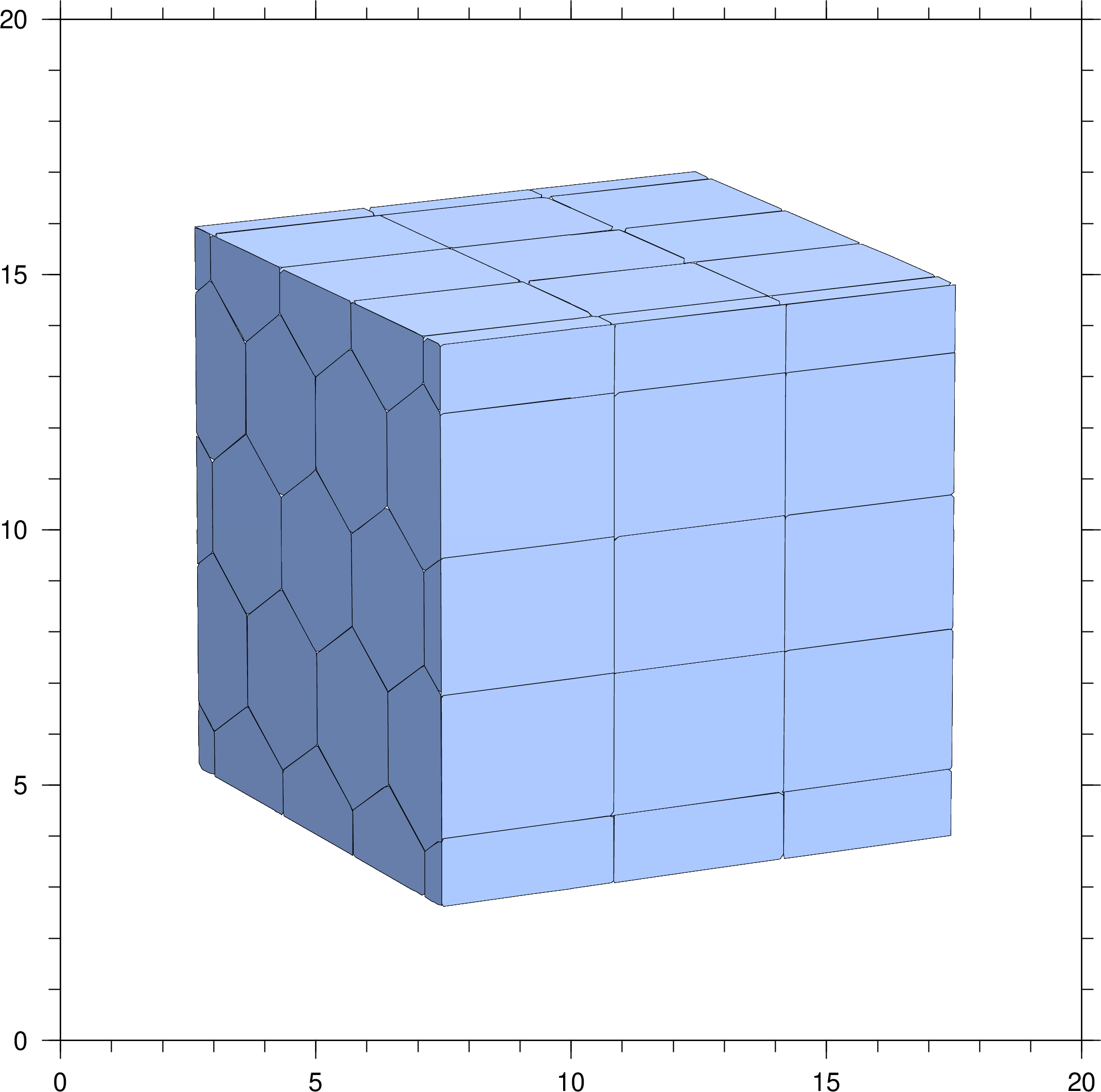
Fig. 5.6.13 Result of [cell] section example (7) in 3D images.
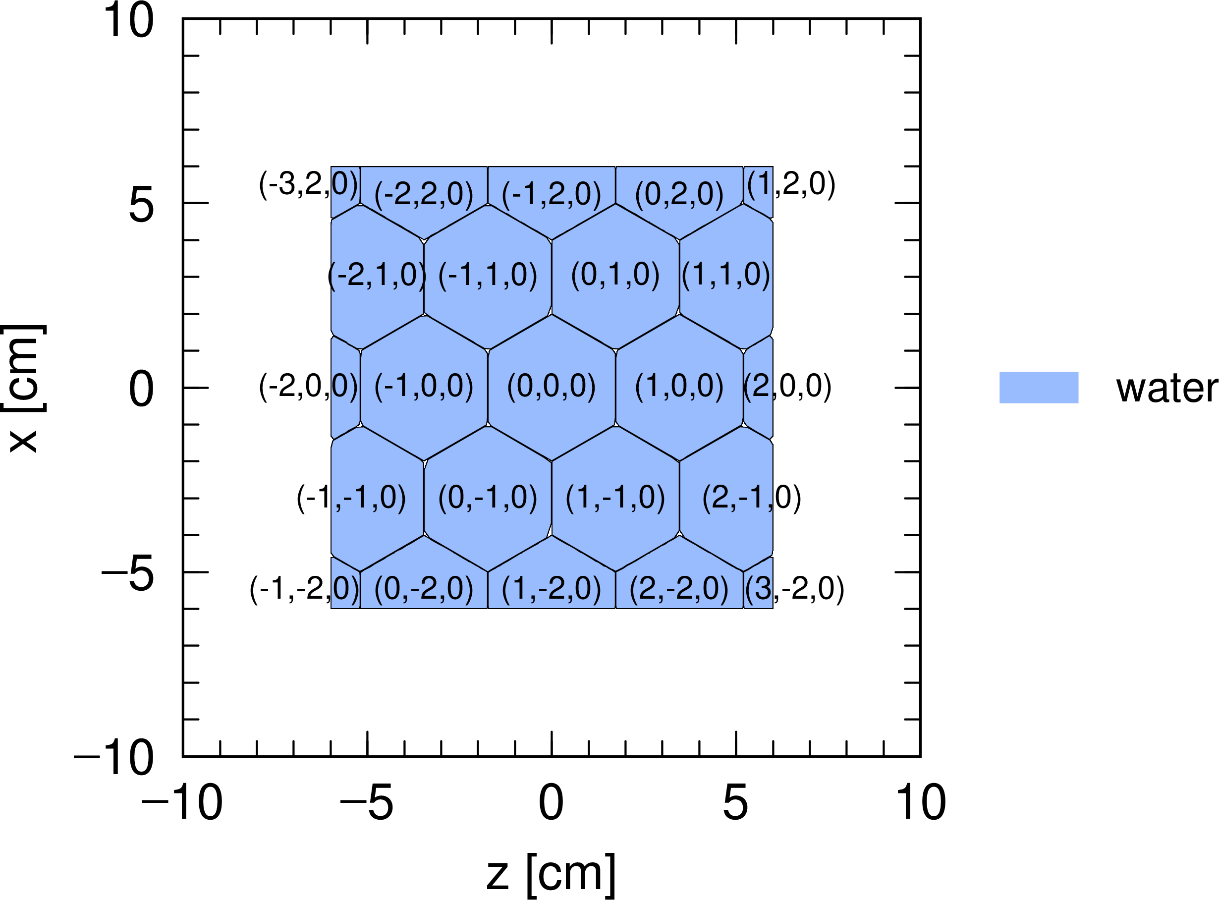
Fig. 5.6.14 Result of [cell] section example (7) in 2D images.
5.6.5. Repeated structures
There are several simple procedures in PHITS that can be used to create repeated structures in which the same or similar units are repeated. Using the lattice parameter described in Section 5.6.4 is one such method; another is the LIKE n BUT cell parameter format.
5.6.5.1. LIKE n BUT cell parameter
Using this format, a cell that differs slightly from an original cell can be created.
In this format, the cell parameters following the BUT statement differ from those in the original cell (n).
The cell parameters that can be used in this format are shown in Table 5.6.2.
In the following example, two cell parameters, TRCL and MAT, are used.
     1:   [ Material ]
     2:     mat[1]  1H 2  16O 1
     3:     mat[2]  Fe 1
     4:   [ Cell ]
     5:       1   0       -10  13 -14  #2 #3 #4
     6:       2   1  -1.0   11 -12  13 -14  15 -16
     7:       3   LIKE 2 BUT  TRCL=1
     8:       4   LIKE 2 BUT  TRCL=2  MAT=2
     9:       5  -1        #(-10  13  -14)
    10:   [ Surface ]
    11:     10  CY   10
    12:     11  PX  -2
    13:     12  PX   2
    14:     13  PY  -2
    15:     14  PY   2
    16:     15  PZ  -2
    17:     16  PZ   2
    18:   [ Transform ]
    19:   *tr1   3 0 -5
    20:   *tr2  0 0 6  0 30 0  0 0 0  0 0 0  2
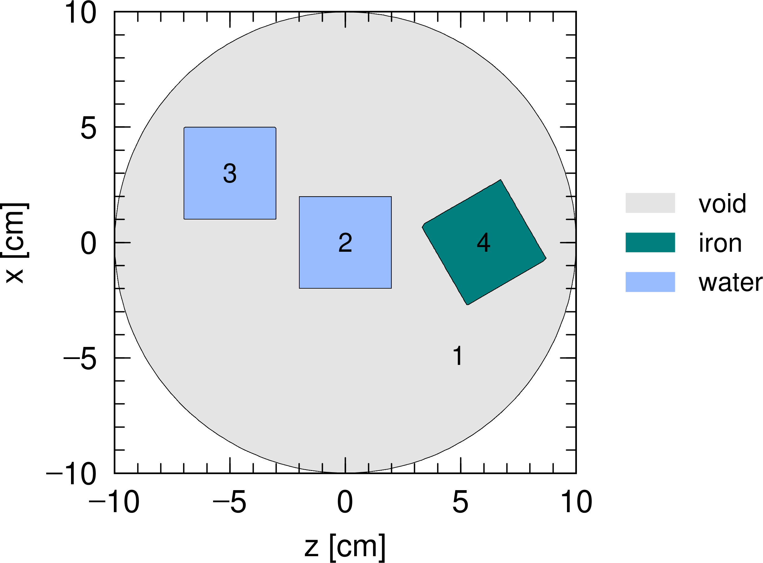
Fig. 5.6.15 Result of [cell] section example (8).
A 4 cm cube filled with water and placed at the origin of the coordinate system is defined in the sixth line.
The interior of this cube is the second cell, which is regarded as the original cell in this example.
In the seventh and eighth lines, respectively, the third and fourth cells are defined using the LIKE n BUT format with n=2.
Fig. 5.6.15 shows the result of this example.
The coordinate system of the third cell is transformed using the cell parameter TRCL=1, where the coordinate transform number 1 is defined in the nineteenth line of the [transform] section.
The coordinate system of the fourth cell is transformed using TRCL=2 and the interior material of the cell is replaced with iron defined using the material number 2 in the third line.
5.6.5.2. Nesting structure with lattice
A nesting structure can be used based on the universe frame described in Section 5.6.3.
For example, universe 1 can be filled with universe 2, and universe 2 can be filled with universe 3, with this process continued following a user-defined nesting structure.
The maximum number of nestings is 10, which corresponds to the parameter mxlv given in the file param.inc.
In the next example, there are nine square poles defined using LAT=1; three of these have unique structures.
     1:   [ Material ]
     2:     mat[1]  1H 2  16O 1
     3:     mat[2]  Fe 1
     4:   [ Cell ]
     5:       1   0        11  -12   13  -14  15  -16  FILL=1
     6:     101   0       -26   25  -22   21  LAT=1  U=1
     7:                   FILL=-1:1  -1:1  0:0
     8:                   2 2 3  2 3 2  3 2 2
     9:     201   1  -1.0  -90  U=2
    10:     301   2 1-0.0  -10  U=3
    11:     302   0        10  U=3
    12:       2  -1       #1
    13:   [ Surface ]
    14:     10  CY   1.5
    15:     11  PX  -6
    16:     12  PX   6
    17:     13  PY  -6
    18:     14  PY   6
    19:     15  PZ  -6
    20:     16  PZ   6
    21:     21  PX  -2
    22:     22  PX   2
    23:     25  PZ  -2
    24:     26  PZ   2
    25:     90  BOX  -10 -10 -10  20 0 0  0 20 0  0 0 20
The definition of the first cell in the fifth line and the lattice unit in the sixth line are the same as in the [cell] section example (6).
However, the format of the cell parameter FILL in the seventh and eighth differs: in the seventh line, regions treated in this calculation are given in the lattice coordinate system.
The numbers in the next line correspond to the universe number filling each lattice at \((i,j,k)\) following the order \((-1, -1, 0), (0,-1,0), (1,-1,0), (-1,0,0), \ldots, (1,1,0)\); in other words, a lattice at \((-1,-1,0)\) is filled with universe 2 and one at \((1,-1,0)\) is filled with universe 3.
Universe 2 is defined in the ninth line as a space filled with water, while the universe 3 is defined in the tenth and eleventh lines has an iron cylinder centered at the origin.
The result of this example is shown in Fig. 5.6.16, in which it can be seen that three lattices at \((1,-1,0)\), \((0,0,0)\), and \((-1,1,0)\) have an iron cylinder.
Specifying a cell using mesh=reg in the tally sections can be done using the lattice and universe styles as (302 < 101[0 0 0]), where the lattice coordinate is represented by [i j k]: see Sec. Volume definition for more information on this format.
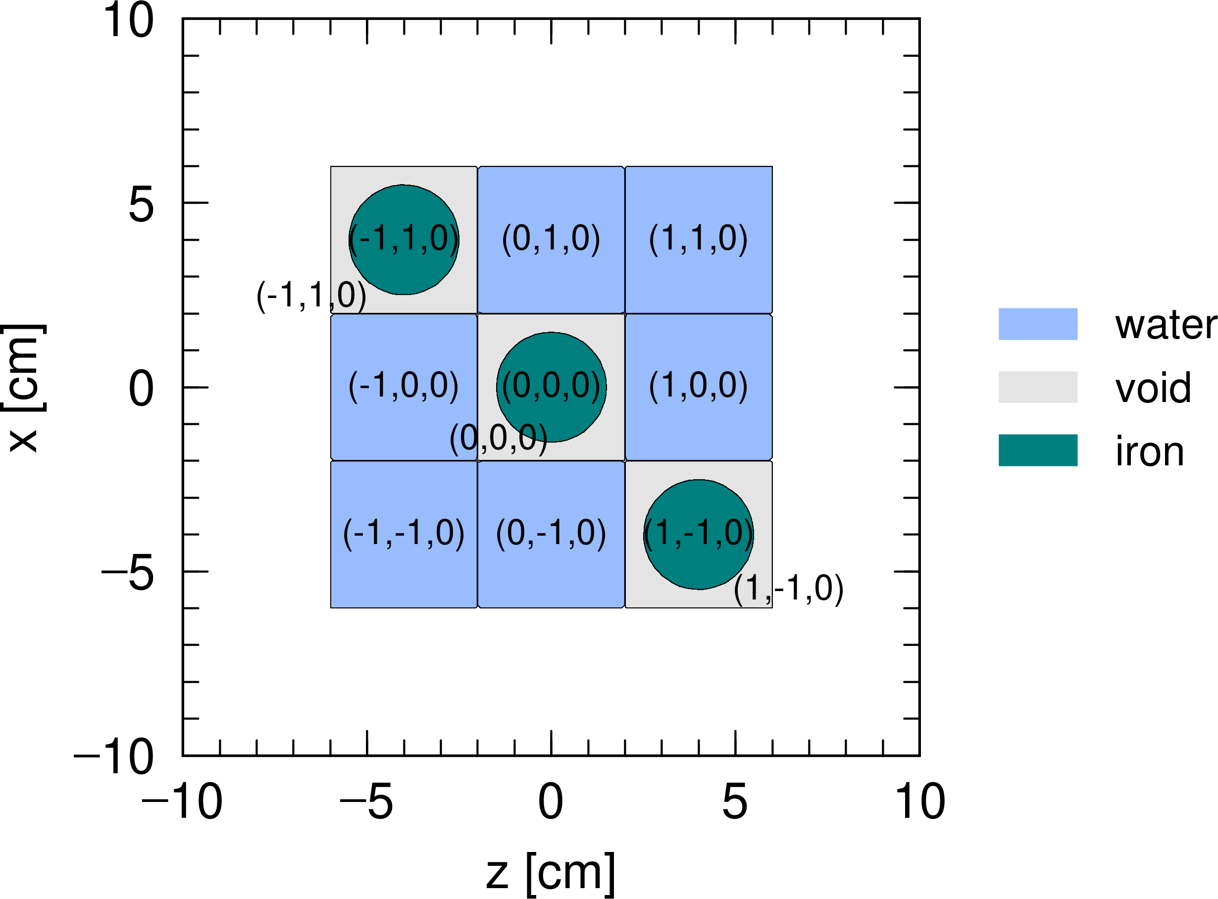
Fig. 5.6.16 Result of [cell] section example (9).
A more complex example is shown below.
     1:   [ Material ]
     2:     mat[1]  1H 2  16O 1
     3:     mat[2]  Fe 1
     4:   [ Cell ]
     5:       1   0        11  -12   13  -14  15  -16  FILL=1
     6:     101   0       -26   25  -22   21  LAT=1  U=1
     7:                   FILL=-1:1  -1:1  0:0
     8:                   2 2 3(1 0 1)  2 3(1 0 1) 2  3(1 0 1) 2 2
     9:     201   1  -1.0  -90  U=2
    10:     301   0       -36   35  -32   31  LAT=1  U=3
    11:                   FILL=-1:0  -1:0  0:0
    12:                   4 2  2 4
    13:     401   2 -10.0  -10  U=4
    14:     402   0        10  U=4
    15:       2  -1       #1
    16:   [ Surface ]
    17:     10  CY   0.5
    18:     11  PX  -6
    19:     12  PX   6
    20:     13  PY  -6
    21:     14  PY   6
    22:     15  PZ  -6
    23:     16  PZ   6
    24:     21  PX  -2
    25:     22  PX   2
    26:     25  PZ  -2
    27:     26  PZ   2
    28:     31  PX  -1
    29:     32  PX   1
    30:     35  PZ  -1
    31:     36  PZ   1
    32:     90  BOX  -10 -10 -10  20 0 0  0 20 0  0 0 20
The virtual space formed by this input is shown in Fig. 5.6.17, in which there are nine square poles defined using the lattice parameter.
Three of the poles comprise four units of the other lattice.
In the eighth line, (1 0 1) denotes a transformation of the coordinate system in which the origin is shifted by 1 cm in both the \(x\)- and \(z\)-directions.
The lattice and universe styles (402 < 301[-1 -1 0] < 101[0 0 0]), where the lattice coordinate is represented as [i j k], can be used to specify any cell using mesh=reg in the tally sections: see Sec. Volume definition for more information on this format.
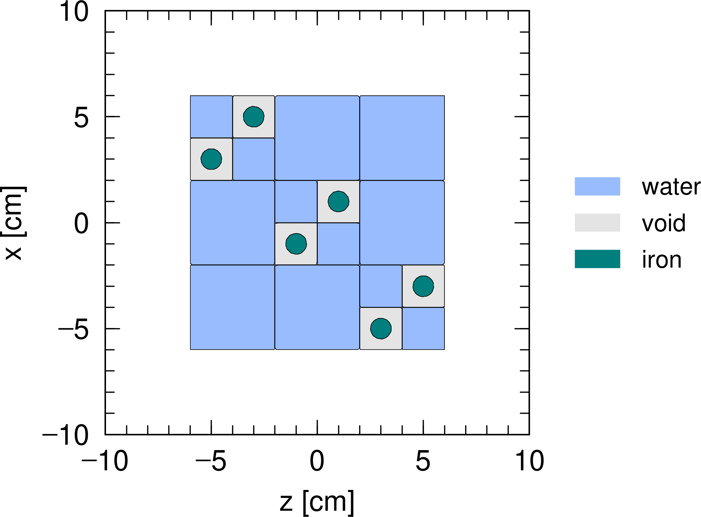
Fig. 5.6.17 Result of [cell] section example (10).
5.6.5.3. Voxel phantom
In PHITS, a virtual space can be created using voxel phantoms for calculation on complex structures such as the human body or an organism. To define a voxel phantom, a small cube must first be defined as the unit of a lattice with LAT=1. This unit is then repeated to define a large-size structure. Each unit can then be filled with a universe, which itself is filled with biological matter, e.g., compounds of carbon and water.
In the example below, a 10-cm cube comprising 125 (\(5 \times 5 \times 5\)) 2 cm cubes (voxels) is described.
     1:   [ Material ]
     2:     mat[1]  1H 2  16O 1
     3:     mat[2]  Fe 1
     4:   [ Cell ]
     5:       1   0   11  -12   13  -14  15  -16  FILL=1
     6:     101   0  -20  LAT=1  U=1
     7:              FILL=-2:2  -2:2 -2:2
     8:              2 2 2 2 2  2 2 2 2 2  2 2 3 2 2  2 2 2 2 2  2 2 2 2 2
     9:              2 2 2 2 2  2 3 3 2 2  2 3 4 3 2  2 3 3 2 2  2 2 2 2 2
    10:              2 2 2 2 2  2 3 3 3 2  3 4 4 4 3  2 3 3 3 2  2 2 2 2 2
    11:              2 2 2 2 2  2 2 3 3 2  2 3 4 3 2  2 2 3 3 2  2 2 2 2 2
    12:              2 2 2 2 2  2 2 2 2 2  2 2 3 2 2  2 2 2 2 2  2 2 2 2 2
    13:     201   0       -90  U=2
    14:     301   2 -10.0  -90  U=3
    15:     401   1  -1.0  -90  U=4
    16:       2  -1       #1
    17:   [ Surface ]
    18:     11  PX  -5
    19:     12  PX   5
    20:     13  PY  -5
    21:     14  PY   5
    22:     15  PZ  -5
    23:     16  PZ   5
    24:     20  BOX  -1 -1 -1  2 0 0  0 2 0  0 0 2
    25:     90  BOX  -10 -10 -10  20 0 0  0 20 0  0 0 20
As the voxel unit, the 2 cm cube is defined in the twenty fourth line.
The first cell, which is located within a 10-cm cube, has a repeated structure as defined in the fifth line.
The region of the lattice coordinate space is determined in the seventh line.
The order of voxels in the eighth through twelfth lines is as follows: \((-2, -2, -2), (-1,-2,-2), \ldots, (2,2,2)\), which represent the lattice coordinates.
In the eighth through twelfth lines, 2 means universe 2, which is void, while 3 and 4 correspond to universes 3 and 4, which are of iron and water, respectively.
Fig. 5.6.18 shows the results of this example, a distorted iron box with regions of water within.
To specify any cell using mesh=reg in tally sections, the lattice and universe styles (401 < 101[0 0 0]), where the lattice coordinate is represented by [i j k], can be used: see Sec. Volume definition for more information.
Note that formats such as, e.g., (301 < 101[-2:2 -2:2 -2:2]) cannot be used because not all 101[-2:2 -2:2 -2:2] cells have a 301st cell.
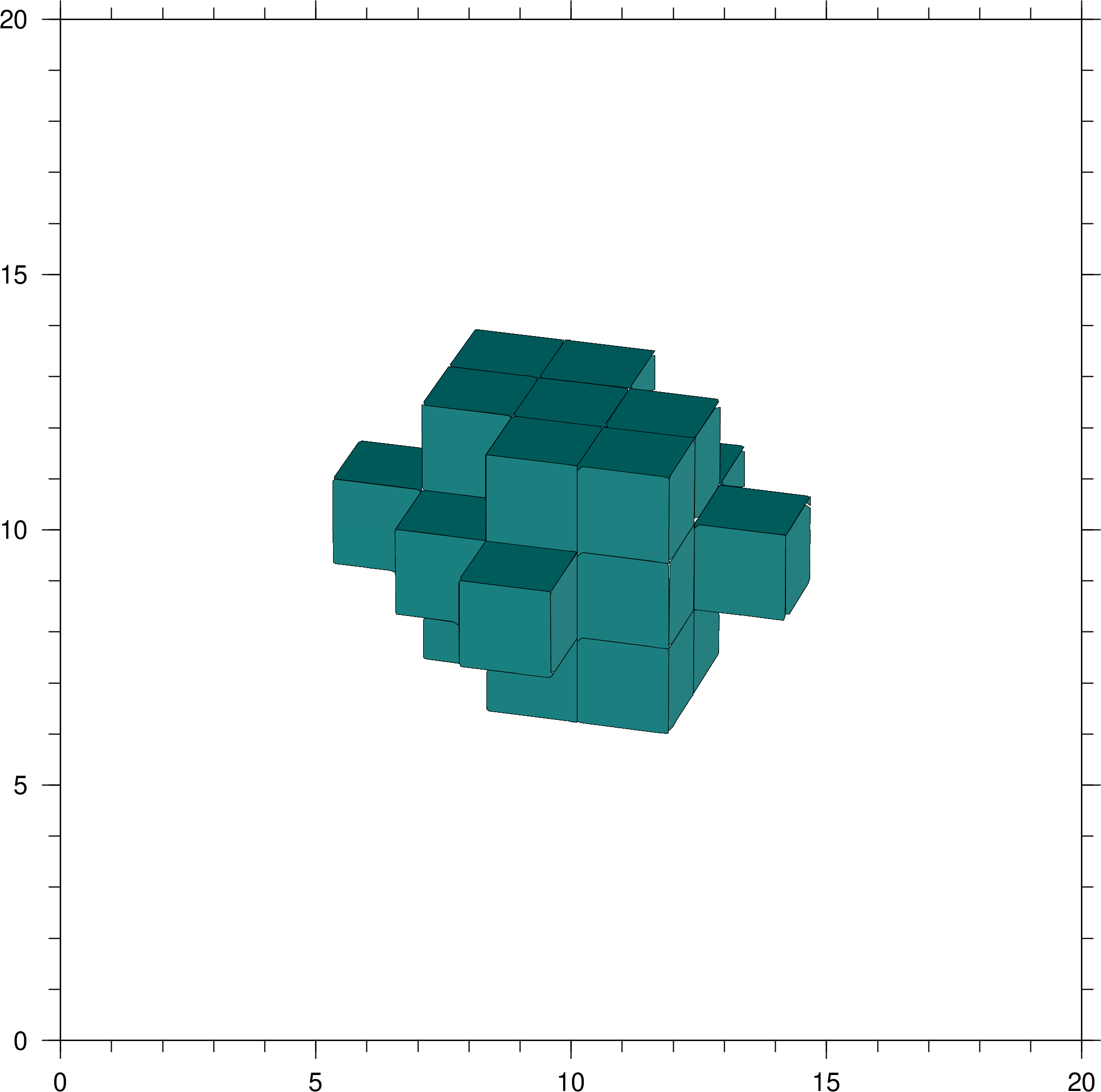
Fig. 5.6.18 Results of [cell] section example (11) in 3D images.
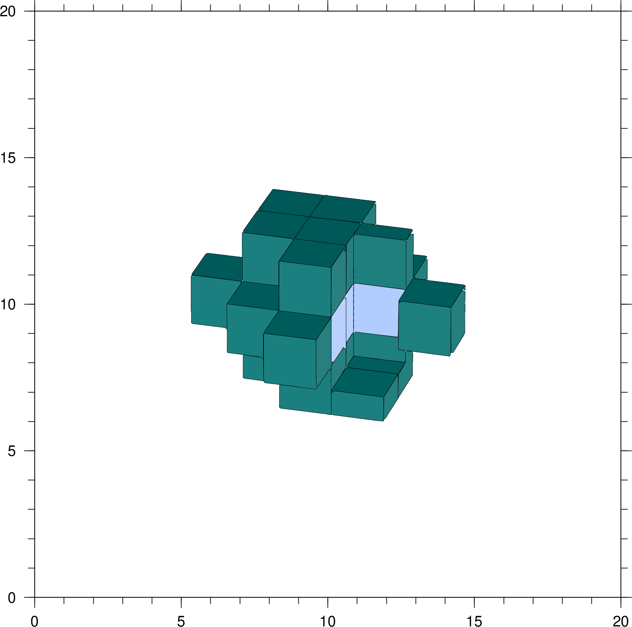
Fig. 5.6.19 Additional 3D view of [cell] section example (11).
From the PHITS version 3.09, the array of universe numbers at the 8th through 12th lines of the example can be expressed in a compressed format. For voxel phantoms, the universe array contains long queues of identical universe numbers, and the compressed format is designed to reduce the size of this array. Thus, reduction of the file size and computational time for reading and writing huge voxel data can be achieved. In the compressed format, arrays of continuous identical universe numbers are given by the number of the repeated universe with a minus sign followed by the universe number. Following this rule, the array of universe number at the 8th through 12th lines of the example can be rewritten as follows.
     8:             2 -11 3 2 -17 3 -1 2 -2 3
     9:             4 3 2 -1 3 -1 2 -12 3 -2
    10:             2 3 4 -2 3 2 3 -2 2 -12 3
    11:             -1 2 -1 3 4 3 2 -2 3 -1 2
    12:             -17 3 2 -11
In the example above, after universe number 2 appears 12 times, universe number 3 comes. On the other hand, the second number -11, which comes after the first number 2, specifies that universe number 2 given before is replicated 11 times afterward.
To save computational time, ivoxel can be specified in the [parameters] section. Performing PHITS calculation with ivoxel=2 causes voxel data to be output in binary to file(18) and then stops the calculation. From the next calculation with ivoxel=1, data output is omitted, which reduces the calculation time. If a very large amount of voxel data is used, it may be more convenient to use infl.
Note that, when ivoxel=1 is specified, the infl command written after the fill specification is automatically skipped by design (the same applies to icells=1). It is therefore not necessary to comment out the infl command when ivoxel=1 is used. Rather, PHIG-3D reads the voxel data from the input file and not from the binary file, so deleting or commenting out the infl command causes an error when the geometry is displayed with PHIG-3D. It is recommended to keep the infl command in the input file even when ivoxel=1 is specified.
5.6.5.4. Use of tetrahedron geometry
In this section, a definition and the basic usage of tetrahedron geometry are given using an example. Tetrahedron geometry is a type of polygon mesh geometry that can express complex geometries by combining tetrahedrons of varying sizes. Note that the function of the reflection boundary does not work in tetra-mesh geometry. Instead by preparing a physically meaningless thin region in the tetra-mesh geometry and defining reflection boundary inside, the reflection boundary in tetra-mesh geometry can be realized.
PHITS adopts two tetrahedron geometry formats. One is the format for the tetrahedral mesh generator, TetGen and the other is the format for the finite element analysis program NASTRAN.
The TetGen format is represented by two files:
the node file (a list of the xyz space coordinates of the tetrahedron nodes)
the element file (a list of four node IDs for each tetrahedron element)
In PHITS, the node and the element files have a common name with different suffixes, .node and .ele, respectively: please refer to the ppt file or sample input file in phits/lecture/advanced/TetraGEOM for a more detailed explanation.
Examples of a node file and an element file are given below.
     1:   # Simple two elements
     2:   5   3  0  0
     3:   #  pointID x y z
     4:   1    0.0  -2.5  -4.0
     5:   2   -4.0  -2.5   0.0
     6:   3    4.0  -2.5   0.0
     7:   4    0.0  -2.5   4.0
     8:   5    0.0   2.5   0.0
The node file begins with the number of nodes and the number of dimensions (second line). PHITS operates only in three-dimensional geometry, and the two last zeros in the second line are not used in PHITS. The following lines (below the third line) represent a list of nodes and their xyz space coordinates in the order
[node no.] [x] [y] [z]
     1:   # Simple two elements
     2:   2  4  1
     3:   # elementID point(1:4) universe
     4:   1     1  2  3  5    1001
     5:   2     5  2  3  4    1002
The element file begins with the number of elements, the number of nodes comprising a tetrahedron (= 4 in PHITS), and the number of information points tagged to the element (=1 in PHITS) [second line]. The following lines (below the third line) give a list of 4-node IDs, each corresponding to a tetrahedron, in the order
[element no.] [node 1] [node 2] [node 3] [node4] [element universe no.]
The element no. represents the ID of the tetrahedron element. The node no. specifies the list of 4-node IDs in the node file. The element universe no. specifies the universe used to fill the tetrahedron element; the definition of this universe should be given in the PHITS input file (See Example). Arbitrary comment lines starting with # can be inserted into any line of the node or element file.
The node and element files can be created using the Tetrahedral Mesh Generator (TetGen) software, which can convert general polygon mesh data to tetrahedron geometry with some effort. TetGen can be obtained free of charge from the following source: TetGen For details on TetGen, please refer to the manual in the link above.
PHITS adopts another format, which is the bulk data format of NASTRAN.
This format is a generally accepted in many software of structural analysis and computational fluid dynamics (CFD).
PHITS uses the bulk data format defined using GRID and CTETRA and assumes those are written in a file with .bdf extension.
The explanation of the buld data format is omitted here because the file will be deduced automatically from some software which is used to create the tetrahedron geometry.
By adopting the same format for the tetrahedral geometry in PHITS as structural analysis or CFD, seamless coupled analysis between those studies and radiation transport calculation becomes possible.
For the details, see a document uploaded in the folder phits utility FLUENT which explains how to conduct such a coupled analysis.
The method for using tetrahedron geometry in a PHITS input file is explained below.
     1:   [Material]
     2:   mat[1] 14N 78.1  16O 20.9  40Ar 0.93
     3:   mat[2] 1H 2  16O 1
     4:   mat[3] 56Fe 1
     5:   [Surface]
     6:   10  rpp   -5.0  5.0  -3.0  3.0  -5.0  5.0
     7:   20  rpp   -7.0  7.0  -5.0  5.0  -7.0  7.0
     8:   90  so     500.0
     9:   [Cell]
    10:   101   1 -0.001205 -20  U=1  LAT=3  tfile=Tetra  TSFAC=1.0
    11:     1   0           -10  FILL=1
    12:     2  -1            10
    13:   201   2 -1.0      -90  U=1001
    14:   202   3 -7.874    -90  U=1002
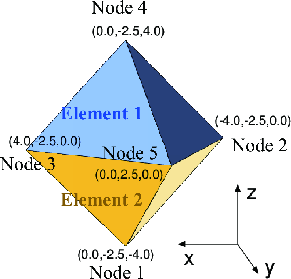
Fig. 5.6.20 Results of [cell] section example (12) in 3D images.
10: 101 1 -0.001205 -20 U=1 LAT=3 nfile=Tetra.bdf TSFAC=1.0
10: 101 1 -0.001205 -20 U=1 LAT=3 hfile=Tetra.ph5 TSFAC=1.0
To use tetrahedron geometry, a region must be defined as a rectangular shape (using the surface symbol RPP).
This region should contain all of the nodes of the tetrahedrons that will be created but should not be so large that it incurs unnecessary computational costs.
At the tenth line in the example code, a region with cell no. 101 is defined as a rectangular shape specified by surface number 20 as a 14 cm \(\times\) 10 cm \(\times\) 14 cm rectangular box.
Setting the LAT option =3 declares the use of a tetrahedron geometry defined by the node and element files with names specified by TFILE.
For a file of the NASTRAN bulk data format, the name should be specified accompanied by NFILE as in example (13).
When specifying NFILE, if the file has a file extension (e.g. .bdf) please specify the file name including the extension. [1]
When using a PHITS HDF5 file in the ph5 format, specify the file name (including its extension) with HFILE instead of TFILE, as in Listing 5.6.17 .
Note that the upper and lower cases of the file name differ between Mac and Linux.
Using the TSFAC factor allows the size of the tetrahedron geometry to be scaled up or down by multiplying the coordinates of the nodes by the value of the factor.
The material given in cell 101 is used to fill all of region 101 aside from the tetrahedron interiors.
In the eleventh line the region with cell no. 1 is defined as a rectangular box of dimensions 10 cm \(\times\) 6 cm \(\times\) 10 cm.
Using the FILL option, this region is filled by the tetrahedron geometry of cell no. 101.
The tetrahedron geometry setting (LAT=3) should be used together with the universe and fill nest structures in the same manner as in lattice structure specification; the universes included in the element file should be defined in the same manner as in the lattice structure (this is done in lines 13 and 14 in this example, where element no. 1 is filled by material 2 (water), while element no. 2 is filled by material 3 (iron).
When the number of universes used in the tetrahedron geometry increases, the cost manually creating the cells done in lines 13 and 14 in the example becomes heavy.
By specifying the option itetauto=1 in the parameter section, the cells corresponding to the universes for tetrahedron geometry will be automatically created.
With this option, extreamly large surface no. 5000 and cells from no. 5001 to no. 5000+n are added to those given in the PHITS input file and thus use of those no. should be avoided to use this option, where n is number of universes used in the tetrahedron geometry.
Density of the added cells are automatically defined by reading PSOLID and MAT tabs when a file with the NASTRAN bulk data format is used.
For a TetGen format file, density information should be provided by an external file.
The file name needs to have the common name but with .txt suffix.
The universe number and its density should be specified for each line as shown in the txt file example below.
The addional cells will be provied with the same material no. as the cell.
Error messages as shown in the error message example below will be displayed by executing PHITS without specifying the materials corresponding to the universes in the tetrahedron geometry.
The materials from 5001 to 5000+n should be defined according to these messages.
This automatic process can be verified by cheking the input echo lines in the phits.out file, where the additional surface and cells will be inserted.
     1:   5001 5001 -1.0
     2:   5002 5002 -7.874
*** ERROR : undefined material
  TETRA material (MID):  1001
    should be defined as material ID number:  5001
*** ERROR : undefined material
  TETRA material (MID):  1002
    should be defined as material ID number:  5002
TRCL specification cannot be used for the cell with LAT=3 option.
To apply a coordinate transformation for the tetrahedron geometry, nest structure by universe and fill specification is required and the TRCL option should be specified in the upper level above the cell containing the tetrahedron geometry with LAT=3.
Please refer to the ppt file or sample input file in /phits/lecture/advanced/TetraGEOM for a more detailed explanation.