5.21. [ WW Bias ] section
In the [ww bias] section, minimum values of the weight window defined in [weight window] can be biased for certain regions. This option is useful when the [weight window] parameters for a certain region are biased after automatically generating the [weight window] section by [t-wwg]. Fig. 5.21.1 shows a flowchart of how to perform a transport calculation using [weight window] and [ww bias]. First, generate the [weight window] section by [t-wwg]. If the obtained parameters of [weight window] are enough to effectively use the variance reduction technique, the [ww bias] section is not needed. However, if they are not enough, the variance reduction technique can be used more effectively by biasing the [weight window] parameters for a certain region with [ww bias]. There are two methods to set the [ww bias] section. One is an automatic method using [t-wwbg], which is a Weight Window Bias Generator, and the other is a manual method by a user, which is explained below. For details of [t-wwbg], see Section 7.17. When performing a transport calculation with [ww bias] and [weight window], set icntl=0 and iwwbias=1 in the [parameters] section.
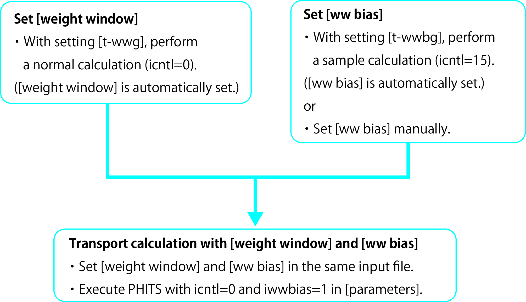
Fig. 5.21.1 The flowchart of the connection calculation between [weight window] and [ww bias].
When more than one [weight window] section is defined, the combinations of [weight window] and [ww bias] are chosen in the order of appearance in the input file. Therefore, the same number of [ww bias] sections are required as the number of [weight window] sections.
The format of [ww bias] is as follows. Note that you should set the same particle, energy mesh, and regions as in [weight window]. mesh=reg is selected as default if the mesh specification is skipped. When mesh=xyz is specified, x-type, y-type, and z-type must be defined in subsequent lines in the same way as for [weight window]. When mesh=tet is specified, the same cell number specification by reg= is required as in [weight window].
    [ WW Bias ]
       part =  neutron
        eng =  2
               1e-3   1.0
        reg    wwb1       wwb2
          1    0.25       0.25
          2    0.50       0.50
          3    1.00       1.00
          4    2.00       2.00
        ....   ........   ........
In the first line, part= defines which particle is to be considered. When it is omitted, part=all is set. The expression of part= is the same as that in tally format. Note that only the expression as ityp can be set. Each nuclide cannot be specified. Next, the energy mesh should be defined. The line starting with eng= specifies the number of meshes. In the next line, energies, \(e_1, e_2, e_3, ...\), are defined. Furthermore, names of columns are given as reg, wwb1, wwb2, and so on. In the reg column, cell numbers are written. Bias values are given in the columns of wwbi. The skip operator non can be used. Each wwbi column corresponds to energies of \(e_{i-1} < E < e_i\). Here, \(e_0=0\) is assumed. The format ( { 2 - 5 } 8 9 ) can be used, and the lattice and universe style ( 6 < 10[1 0 0] < u=3 ) can also be used. However, any value that is not a single numeric value must be enclosed by ( ).
By setting iwwbias=1 in the [parameters] section, the [weight window] parameters multiplied by the inverse of the defined biases in [ww bias] are used. In this case, the products of the multiplication are output in the input echo of [weight window], and [ww bias] with off is output. If an input file without [ww bias] is used, all values of [ww bias] in the input echo are set to 1.
An example of [ww bias] is as follows.
     1:   [ WW Bias ]
     2:      part = neutron
     3:       eng =  1
     4:            1.00000E+05
     5:
     6:      reg       wwb1
     7:      1         1/7
     8:      2         1/6
     9:      3         1/5
    10:      4         1/4
    11:      5         1/3
    12:      6         1/2
    13:      7         1
    14:      8         2
    15:      9         3
    16:      10        4
    17:      11        5
    18:      12        6
Here, neutron is considered as part. One energy region below 100 GeV is specified. Regions between 1 and 12 are gradually biased. The region with a larger number is biased more strongly than that with a smaller number.
The xz cross-sectional view of a geometry, a concrete cylinder with a central axis on the z-axis and a radius of 100 cm, is shown below. Two results of neutron fluence obtained by transport calculations without and with [ww bias] are also shown below. Source particles of 14 MeV neutrons were generated at x=0, y=0, z=90 cm as an isotropic source. After generating a [weight window] section by [t-wwg], the result without [ww bias] was obtained by performing the calculation with only the [weight window] section. The result of the calculation with both the [weight window] section and the [ww bias] section of Listing 5.21.2 is also shown below. The neutron fluence without [ww bias] was distributed in both regions of small and large cell numbers. On the other hand, the fluence with [ww bias] was distributed only in the large cell numbers, which were biased by [ww bias] of Listing 5.21.2. As seen in this example, when focusing on a certain region, the calculation can be efficiently performed by [ww bias].
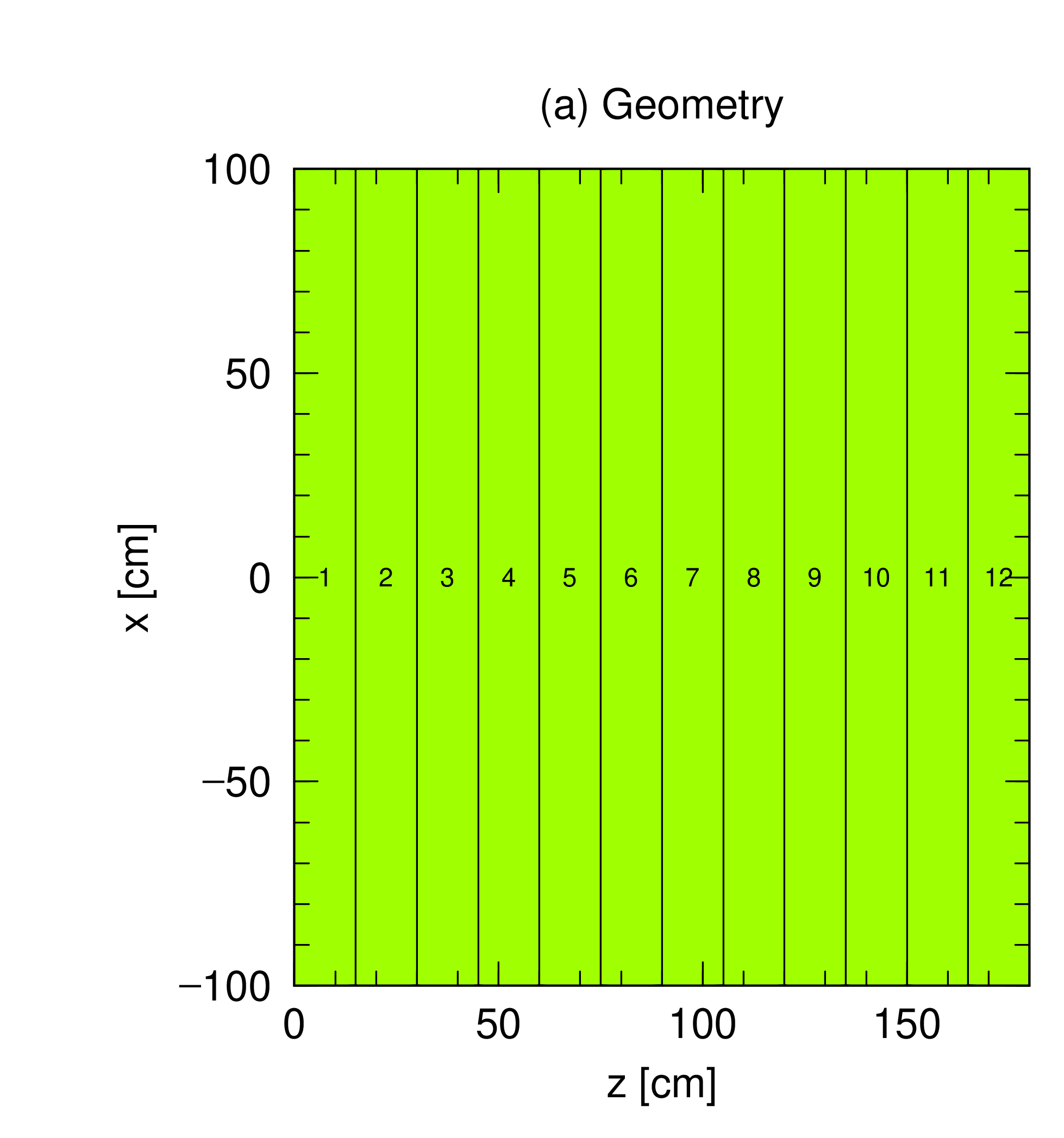
xz cross-sectional view of the geometry.
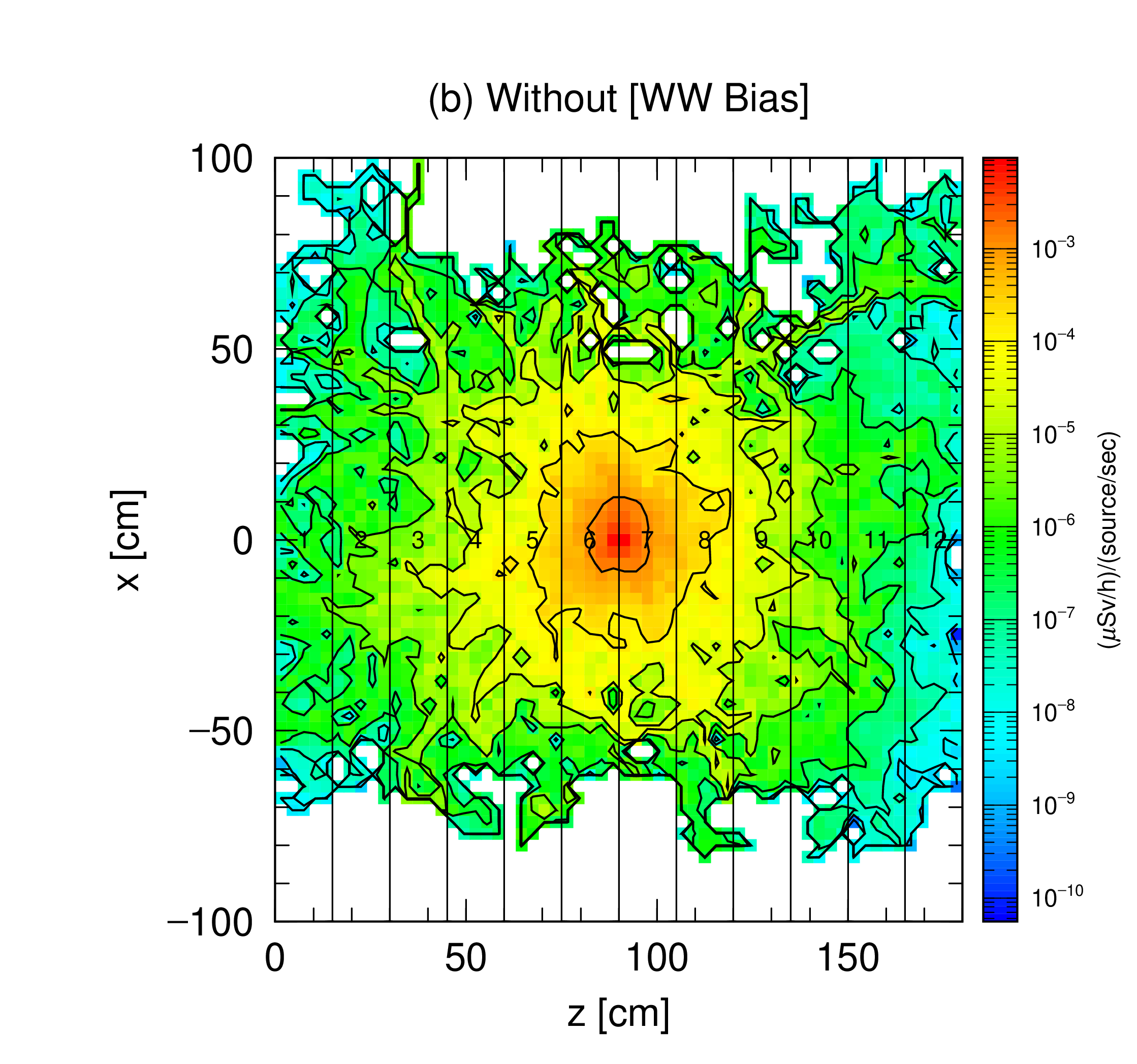
Result without [ww bias].
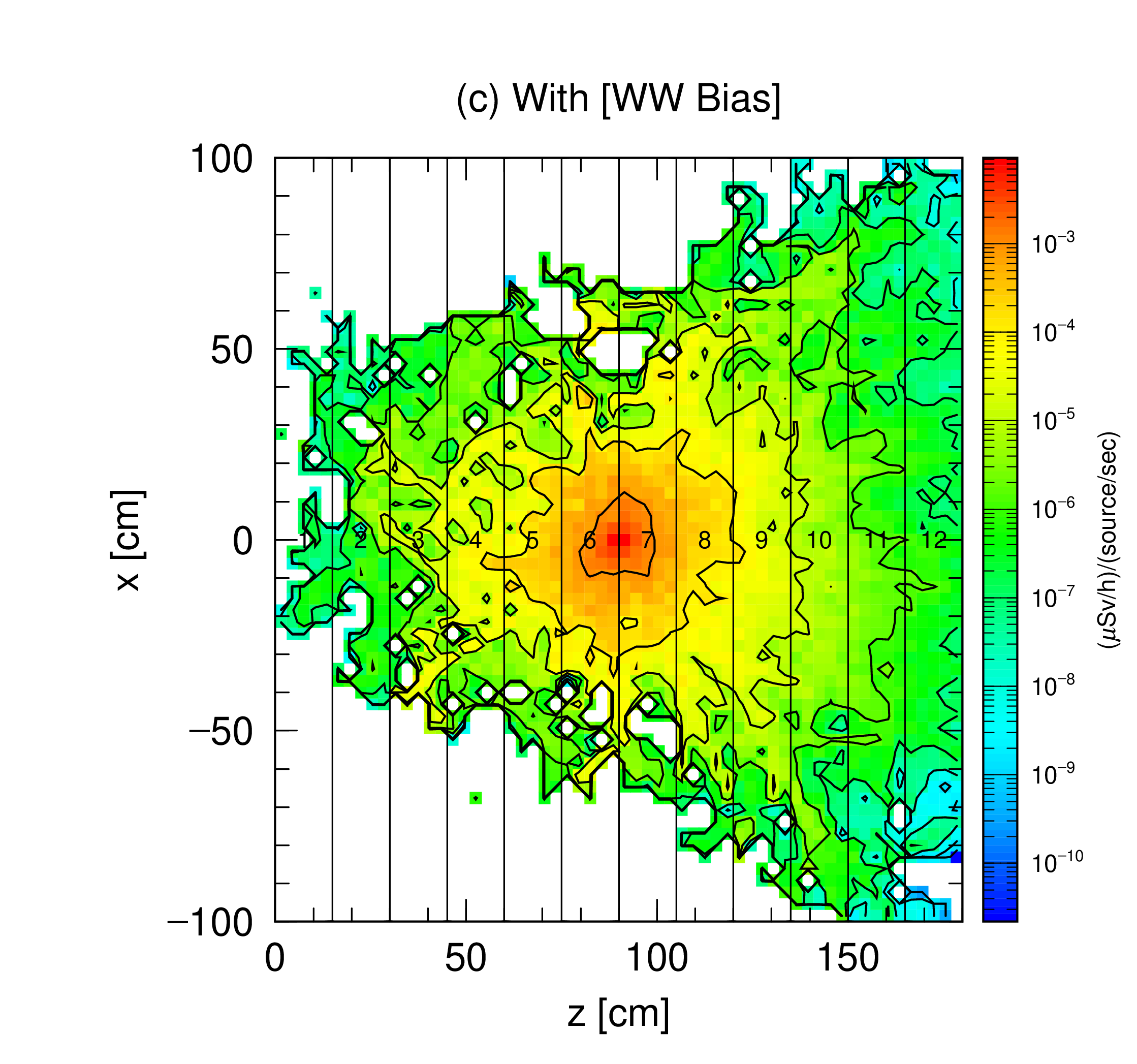
Result with [ww bias] of Listing 5.21.2.