5.11. [ Electro Magnetic Field ] section
Electric and magnetic fields in any region can be set. By defining parameters in this section and setting ielctf=1 in the [parameters] section, PHITS can simulate motion of a charged particle in the fields. To use this function for electrons and positrons, set EGS5 mode. Except for quadrupole magnetic field and magnetic fields for neutrons, both electric and magnetic fields can be set.
5.11.1. Uniform electric and magnetic fields
When using uniform electric and magnetic fields, set the parameters as follows.
[ Electro Magnetic Field ]
  reg   elf   mgf   trcle   trclm
  1     100   1     1       2
  2     100   1     1       2
Cell number (reg), strength of the electric and magnetic fields (elf and mgf, respectively), and directions of the two fields (trcle and trclm) should be defined. The units of elf and mgf are kV/cm and kGauss, respectively. The coordinate transformation numbers defined in the [transform] section should be set to trcle and trclm. When trcle=0, the direction of the electric field is the positive x-axis. When trclm=0, the direction of the magnetic field is the positive y-axis. trcle and trclm are not omissible. When elf or mgf is set to 0, or when the transformation is not used, trcle and trclm should be set to 0.
When typm or type are not defined, parallel electric field and parallel (dipole) magnetic field are assumed:
[ Electro Magnetic Field ]
  reg   elf   typm  mgf   trcle   trclm
  1     0     4     10    0       1
  2     0     2     1     0       2
typm is a magnetic field type identifier (2 means dipole and 4 means quadrupole). Quadrupole magnet cannot be combined with electric field. Cell number ( reg ), …, trcle and trclm should be set to 0.
The format ( { 2 - 5 } 8 9 ) can be used. However, any value that is not a single numeric must be enclosed by ( ). The lattice and universe style can be used as ( 6 < 10[1 0 0] < u=3 ). By using this format, different magnetic fields can be set for each lattice. If a cell is re-defined, the value defined first is used.
In the case of a dipole magnet, the distance gap makes no sense, but any numeric value should be set. The magnetic field is available not only in the void region, but also in materials where the normal reaction can occur.
The z-axis is assumed to be the center of the magnetic field. The direction of the magnetic field is the positive y-axis for a dipole, that is, a positively charged particle is bent in the negative x direction when it goes in the positive z direction. For a quadrupole, the positive particle is converged in the x-axis and diverged in the y-axis when it goes in the positive z direction. The coordinate transformation by trcl is needed for different geometrical situations.
When specifying the charge number of the projectile particle with izst in the [source] section, the motion of the particle with that number in the electro-magnetic field is described. Using izst, PHITS can simulate motion of a particle with charge states. The charge number defined with izst does not change while the particle moves. It should be noted that particles produced from nuclear reactions are not affected by the value of izst. The charge of the produced particle is given as its atomic number.
If you want to precisely calculate the trajectory of charged particles under a strong electromagnetic field that significantly bends their trajectories within a short distance less than a few cm, set the maximum flight mesh size (deltg) in the electromagnetic field to a smaller value.
5.11.2. Neutron
The definition of the magnetic field for neutrons is almost the same as that for charged particles. Here we describe the details of the magnetic field for neutrons.
    [ Magnetic Field ]
      reg    typ    gap            mgf           trcl      polar     time
        1     60    0.00000       35000.0          3        non      non
        2     61    0.00000       35000.0          1         1       non
        3    106    5.00000        7130.0          0         0       non
        4    104    0.00000        3.5             0        non      5.0
        5    102    0.00000        0.20            0        non      non
        6    101    3.00000        7130.0          2         1       non
        7    103    0.00000       35000.0          0        -1       non
       ...   ...    ........       ........       ...       ...      ...
       ...   ...    ........       ........       ...       ...      ...
The effects of gravity and an additional dipole magnet cannot be taken into account in the first two cases. For 60, it is assumed that the spin always keeps parallel or anti-parallel to the magnetic field. For 61, PHITS solves the coupled equation of motion between the spin and the magnetic field. Then spin flip can occur in a region with a weak magnetic field. The strength of the magnetic field is specified in the mgf column in units of [T/m \(^2\)].
For types above 100, PHITS considers the coupled equations of the spin and the magnetic field. In addition, the effects of gravity and an additional dipole field can be taken into account. 106 is sextupole, 104 is quadrupole, and 102 is dipole. The strength of the additional dipole magnet in the z-direction is given by the gap column in units of [T].
For 101 type, the magnetic field is defined by the user program file usrmgf1.f90. In this user program, data measured by the neutron optics group in JAERI are read from the file and used in the calculation. The strength of this field is renormalized by the value of mgf.
For 103 type, the magnetic field is also defined by the user program file usrmgf3.f90. In this user program, there is a simple sextupole magnetic field, the same as in 106 type.
The neutron goes into the magnetic field with the initial spin if it is defined in the source section. If not, the initial spin is defined at the moment when the neutron goes into the magnetic field. The ratio of the number of parallel and anti-parallel spins to the magnetic field is determined by the polarization defined by the polar column. non in the polar column means zero polarization. The polarization is defined as
Here, \(\phi_+\) and \(\phi_-\) are the numbers of the parallel and anti-parallel particles.
5.11.3. Implementation of the magnetic field map
Since version 3.10, PHITS can read arbitrary magnetic fields given in xyz or r-z grid data. An example of [ Magnetic Field ] for reading a magnetic field map is shown below.
[ Magnetic Field ]
  reg   typ   gap    mgf   trcl   file
  101   -1    10.0   0.5   0      xyzlist.dat
  102   -2    100.0  3.0   0      rzlist.dat
  103   -3    10.0   10.0  0      xyzmap.dat
  104   -4    1.0    1.0   1      rzmap.dat
Four types of magnetic field maps can be read by PHITS. They are specified by typ=-1 to -4 for charged particles and typ=-101 to -104 for neutrons. Only one magnetic field map can be defined for each type in an input file. The meanings of each type are shown in Table 5.11.1. Please see Section 5.11.4 for more details.
typ |
Explanation |
|---|---|
-1 or -101 |
xyz grid, data list type |
-2 or -102 |
r-z grid, data list type |
-3 or -103 |
xyz grid, data map type |
-4 or -104 |
r-z grid, data map type |
The meanings of gap and mgf are different from those in the case of conventional magnetic fields. Here, gap is inversely proportional to the step size for calculating the particle trajectory. Setting a higher value for gap results in a smoother trajectory but longer computational time. On the other hand, mgf indicates the normalization factor of the field strength for magnetic field map cases. For example, you have to set mgf=10 when your magnetic field map is written in units of T because the unit of magnetic field in PHITS is kG. Note that electron and positron step sizes in the magnetic field are automatically determined irrespective of gap. The name of the magnetic field map file is specified by the file parameter. trcl indicates the transform number applied to the magnetic field map, though it does not work for electron and positron transport simulation in the same manner as the conventional magnetic field.
5.11.4. Format of magnetic field map file
The magnetic field map file should consist of header and data parts. In the header part, comment marks can be inserted using # and $, similarly to the PHITS input file. Examples of magnetic field map files together with the PHITS input files to read them are included in the phitssamplemiscmagmap folder.
5.11.4.1. Header format
In the header part, discrimination between lowercase and uppercase characters is not performed, and blanks are ignored in the same manner as PHITS input. Only one parameter can be specified in one line.
Value |
Explanation |
Not omissible
|
Number of x grid.
Used only for typ=-1 and -3.
|
Value |
Explanation |
Not omissible
|
Number of y grid.
Used only for typ=-1 and -3.
|
Value |
Explanation |
Not omissible
|
Number of z grid.
Used only for typ=-1 and -3.
|
Value |
Explanation |
Not omissible
|
Number of r grid.
Used only for typ=-2 and -4.
|
Value |
Explanation |
(D=0)
|
Minimum value of x grid in cm.
Used only for typ=-3.
|
Value |
Explanation |
Not omissible
|
Maximum value of x grid in cm.
Used only for typ=-3.
|
Value |
Explanation |
(D=0)
|
Minimum value of y grid in cm.
Used only for typ=-3.
|
Value |
Explanation |
Not omissible
|
Maximum value of y grid in cm.
Used only for typ=-3.
|
Value |
Explanation |
(D=0)
|
Minimum value of z grid in cm.
Used only for typ=-3 and -4.
|
Value |
Explanation |
Not omissible
|
Maximum value of z grid in cm.
Used only for typ=-3 and -4.
|
Value |
Explanation |
(D=0)
|
Minimum value of r grid in cm.
Used only for typ=-4.
|
Value |
Explanation |
Not omissible
|
Maximum value of r grid in cm.
Used only for typ=-4.
|
Value |
Explanation |
(D=1)
|
Existence of the \(B_x\) map.
1 means yes and 0 means no.
Used only for typ=-3.
|
Value |
Explanation |
(D=1)
|
Existence of the \(B_y\) map.
1 means yes and 0 means no.
Used only for typ=-3.
|
Value |
Explanation |
(D=1)
|
Existence of the \(B_z\) map.
1 means yes and 0 means no.
Used only for typ=-3 and -4.
|
Value |
Explanation |
(D=1)
|
Existence of the \(B_r\) map.
1 means yes and 0 means no.
Used only for typ=-4.
|
Value |
Explanation |
Omissible
|
Extend the field to negative x.
Used only for typ=-1 and -3.
|
Value |
Explanation |
Omissible
|
Extend the field to negative y.
Used only for typ=-1 and -3.
|
Value |
Explanation |
Omissible
|
Extend the field to negative z.
Used for all typ.
|
Value |
Explanation |
Header terminator
|
End of header.
|
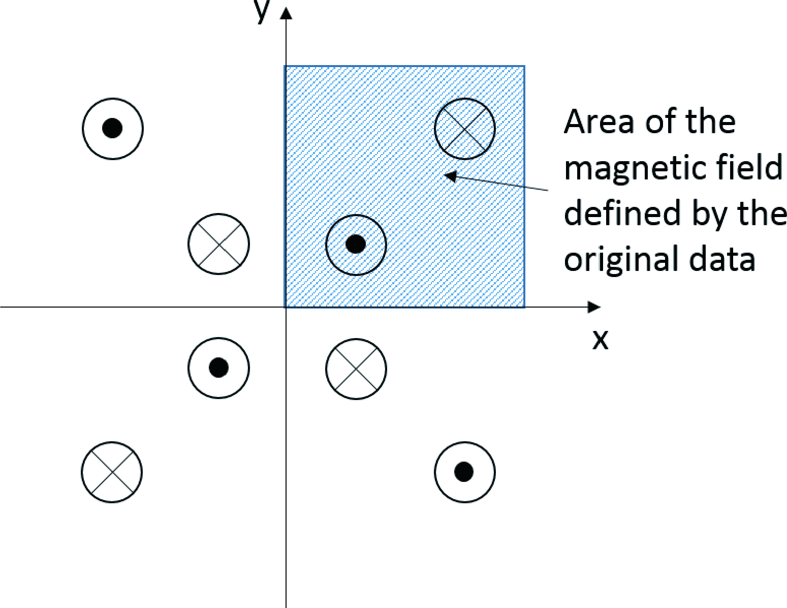
Fig. 5.11.1 Example of the extended magnetic field with the flip command.
If you want to flip the direction of the magnetic field in the extended field, write for example flip=bx, bz, where bx and bz indicate the direction of the magnetic field to be flipped. For example, if you set
extendx flip = bz
extendy flip = bz
the magnetic field for the z-direction (\(B_z\)) is flipped as shown in Fig. 5.11.1. Note that the magnetic fields for the x and y directions are not flipped in this case.
5.11.4.2. Data format
In the data part, only numerical values separated by comma, tab, or blank can be written. Comments cannot be inserted except in columns behind the last numerical data on each line. The units of the grid coordinate and the magnetic field are cm and kG, respectively. Note that the magnetic field strength at the point of each grid should be given instead of that at the center of each grid mesh. The formats of each field type are as follows.
x_1    y_1    z_1    Bx_1,1,1    By_1,1,1    Bz_1,1,1
x_1    y_1    z_2    Bx_1,1,2    By_1,1,2    Bz_1,1,2
...
x_1    y_1    z_nz   Bx_1,1,nz   By_1,1,nz   Bz_1,1,nz
x_1    y_2    z_1    Bx_1,2,1    By_1,2,1    Bz_1,2,1
...
x_1    y_ny   z_nz   Bx_1,ny,nz  By_1,ny,nz  Bz_1,ny,nz
x_2    y_1    z_1    Bx_2,1,1    By_2,1,1    Bz_2,1,1
...
x_nx   y_ny   z_nz   Bx_nx,ny,nz By_nx,ny,nz Bz_nx,ny,nz
r_1    z_1    Br_1,1    Bz_1,1
r_1    z_2    Br_1,2    Bz_1,2
...
r_1    z_nz   Br_1,nz   Bz_1,nz
r_2    z_1    Br_2,1    Bz_2,1
...
r_nr   z_nz   Br_nr,nz  Bz_nr,nz
Bx_1,1,1  Bx_2,1,1  Bx_3,1,1  ...  Bx_nx,1,1
Bx_1,2,1  Bx_2,2,1  Bx_3,2,1  ...  Bx_nx,2,1
...
Bx_1,ny,1  Bx_2,ny,1  Bx_3,ny,1  ...  Bx_nx,ny,1
Bx_1,1,2   Bx_2,1,2   Bx_3,1,2   ...  Bx_nx,1,2
...
Bx_1,ny,nz  Bx_2,ny,nz  Bx_3,ny,nz  ...  Bx_nx,ny,nz
(continue the data for By and Bz in the same format)
 Br_1,1 Br_2,1 Br_3,1 ... Br_nz,1
 Br_1,2 Br_2,2 Br_3,2 ... Br_nz,2
 ...
 Br_1,nr Br_2,nr Br_3,nr ... Br_nr,nz
(continue the data for Bz in the same format)
The order of the data cannot be changed. However, you can omit definition of the field strength for certain directions by specifying ibxmap, ibymap, ibzmap, and ibrmap for typ=-3 and -4. In that case, the field strength for the omitted directions is assumed to be zero. For typ=-1 and -2, the grid coordinates should be given in ascending order. The computational time for data map types is generally shorter than that for the data list type, but they are nearly equivalent when the interval of each grid coordinate is constant.
5.11.5. Use of electric field map
Since version 3.20, PHITS can read arbitrary electro-magnetic fields given in xyz or r-z grid data. The basic format for defining the electro-magnetic field map is the same as that for the magnetic field described in Section 5.11.3, except that filee and type are used instead of file and typ, respectively, to specify the file name and type of electric field. The magnetic field can co-exist with the electric field by specifying its file name and type as filem and typm, respectively. An example of [ Electro Magnetic Field ] for reading the field maps is shown below.
[ Electro Magnetic Field ]
reg  type  typm  gap   elf    mgf  trcle  trclm     filee        filem
102  -3     -1   10.0  100.0  10.0   0      0    xyzmap.dat  xyzlist.dat
type and typm can be defined in the same manner as the magnetic field types shown in Table 5.11.1. Note that type from -101 to -104 cannot be combined with electric fields. From Ver.3.36, this feature now supports multiple field maps ( files ), whereas it was previously limited to a single map per input file. elf and mgf indicate normalization factors of the field strength for the electric and magnetic field maps, respectively. When they are set to 1.0, the electric and magnetic field maps should be given in units of kV/cm and kG, respectively. gap is inversely proportional to the step size for calculating the particle trajectory, that is, setting a higher value for gap results in a smoother trajectory but longer computational time. Note that electron and positron step sizes in the magnetic field are automatically determined irrespective of gap. trcle and trclm indicate the transform numbers applied to the electric and magnetic field maps, respectively, though they do not work for electron and positron transport simulation in the same manner as the uniform electro-magnetic field.
The definition of the electric field map is the same as that of the magnetic field map except for the unit, kV/cm instead of kG. Please refer to Section 5.11.4, “Format of magnetic field map file”, for more details.