5.3.22. Examples of multi-source

Examples of multi-source are shown below. These examples also include energy distributions using functions and an angular-distribution example. First, the list of source sections is shown.

Listing 5.3.3 Example of multi-source

   1:   [ Source ]
   2:    totfact = 3
   3:   <source> = 9.72
   4:     s-type = 1
   5:       proj = proton
   6:         z0 = 2
   7:         z1 = 29
   8:         r0 = 5
   9:         r1 = 4
  10:        dir = 0.0
  11:     e-type = 6
  12:        eg1 = 1.e-6
  13:        eg2 = 1.e-3
  14:        nm  = -200
  15:       set: c10[1.e-4]
  16:       f(x) = x**(1.5)*exp(-x/c10)
  17:   <source> = 1
  18:     s-type = 1
  19:       proj = photon
  20:         z0 = 1
  21:         z1 = 2
  22:         r0 = 5
  23:        dir = -1
  24:     e-type = 5
  25:        eg1 = 1.e-3
  26:        eg2 = 5.e-1
  27:        nm  = 200
  28:        set: c10[1.e-1]
  29:        set: c20[1.e-1/2.35482]
  30:       f(x) = exp(-(x-c10)**2/2/c20**2)
  31:   <source> = 1
  32:     s-type = 1
  33:       proj = neutron
  34:         z0 = 29
  35:         z1 = 30
  36:         r0 = 5
  37:     e-type = 6
  38:        eg1 = 1.e-2
  39:        eg2 = 1.e+3
  40:        nm  = -200
  41:        set: c10[92.469]
  42:        set: c20[5.644e+10]
  43:       f(x) = c10/c20*exp(-sqrt(x*(x+1876))/c10)*(x+938)/sqrt(x*(x+1876))
  44:        dir = data
  45:     a-type = 5
  46:        ag1 = 0
  47:        ag2 = 1
  48:        nn  = 200
  49:       g(x) = exp(-(x-1)**2/0.3**2)

This example contains three sources starting with <source>. The first source is a cylinder with \(z\) from 2 cm to 29 cm and radius 5 cm. However, because r1 = 4 is defined, the inner region of radius 4 cm is excluded. Thus, it is a hollow cylindrical source. The next source is also a cylinder of radius 5 cm, with a thickness of 1 cm from \(z=1\) cm to 2 cm. The last source is the same thin cylinder as the previous one, but with \(z\) from 29 cm to 30 cm. The values defined by <source> for each source are the relative ratios of the sources. Here, they are set to the volume ratios of each source. Therefore, in this multi-source setting, particles are generated uniformly in the defined source regions. The coordinate distribution calculated by [t-product] with output = source and icntl = 6 is shown below. This source defines a 1-cm-thick surface region of a cylinder.

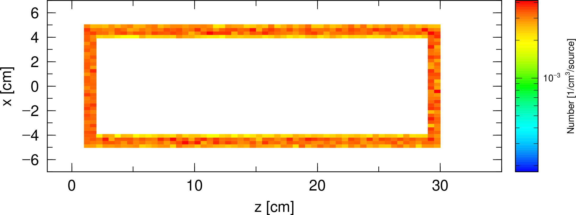
Fig. 5.3.7 Multi-source, spatial distribution

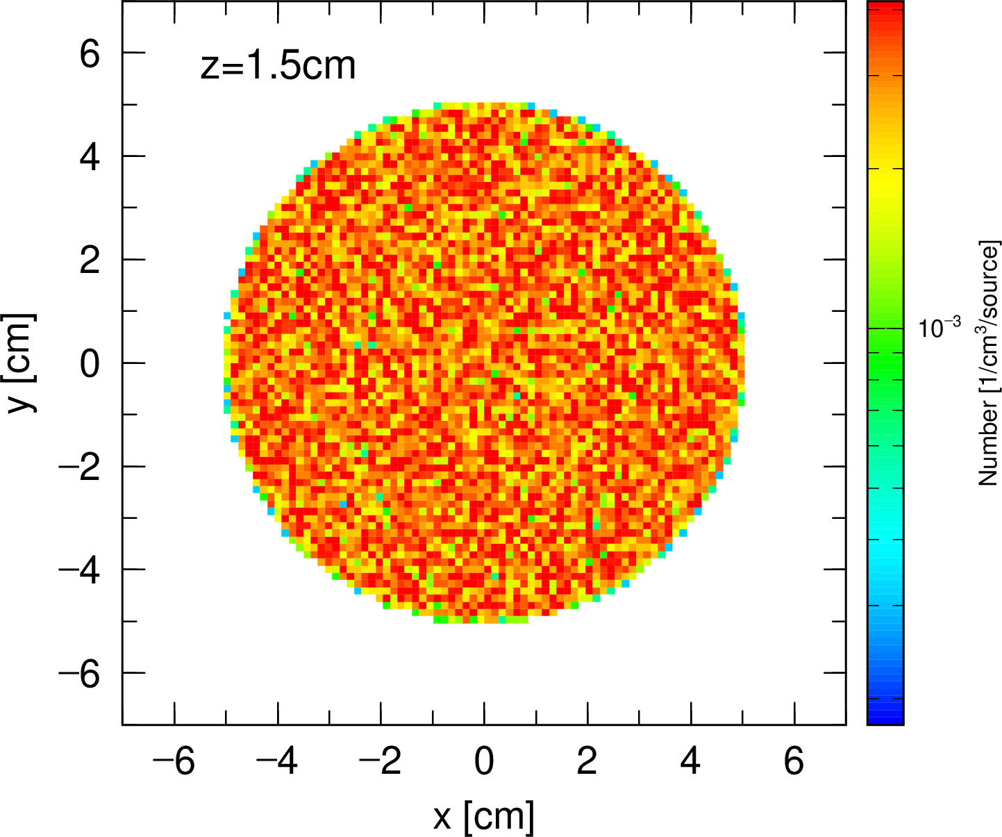
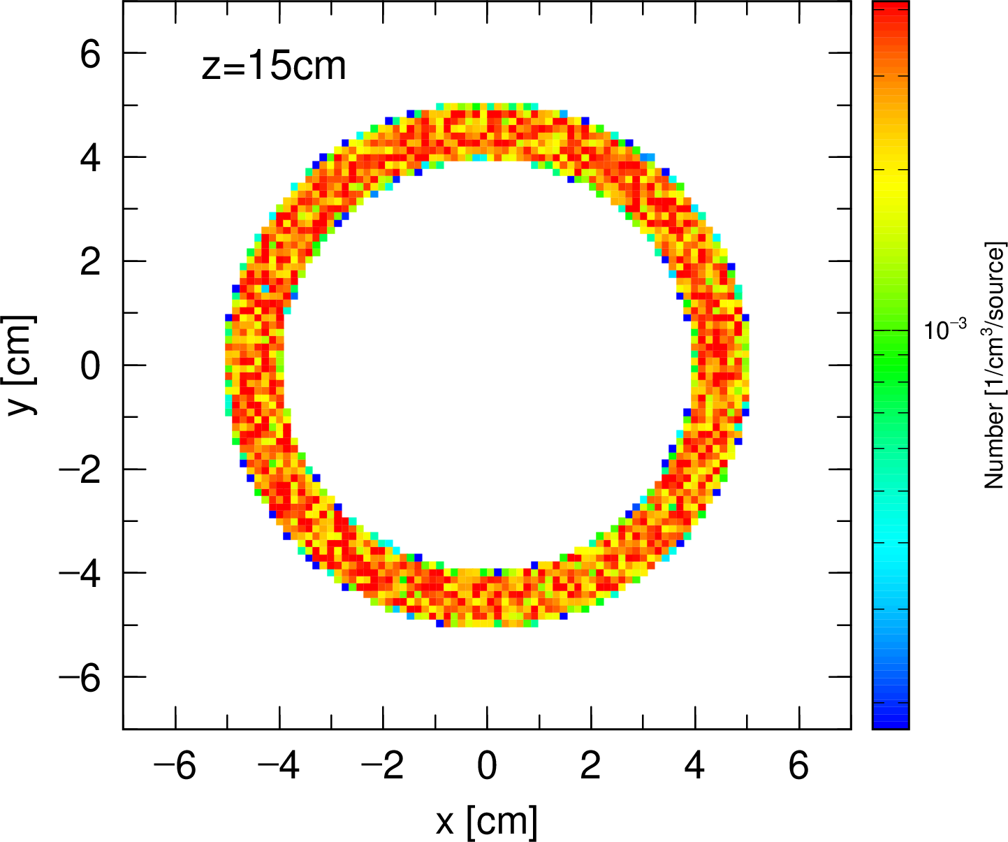
Next, the three source particles are proton, photon, and neutron. Their energy distributions are defined by functions. The first is a Maxwell distribution, the second is a Gaussian distribution, and the last is an arbitrary function. The first Maxwell distribution is equivalent to e-type=7 with

e-type = 7
  et0 = 1.e-4
  et1 = 1.e-6
  et2 = 1.e-3

The second Gaussian distribution is equivalent to e-type=2 with

e-type = 2
  eg0 = 1.e-1
  eg1 = 1.e-1
  eg2 = 1.e-4
  eg3 = 5.e-1

These energy distributions calculated by [t-product] with output=source, icntl=6 are shown below. The results are plotted for each particle, so the energy distribution of each source is shown in a different color.

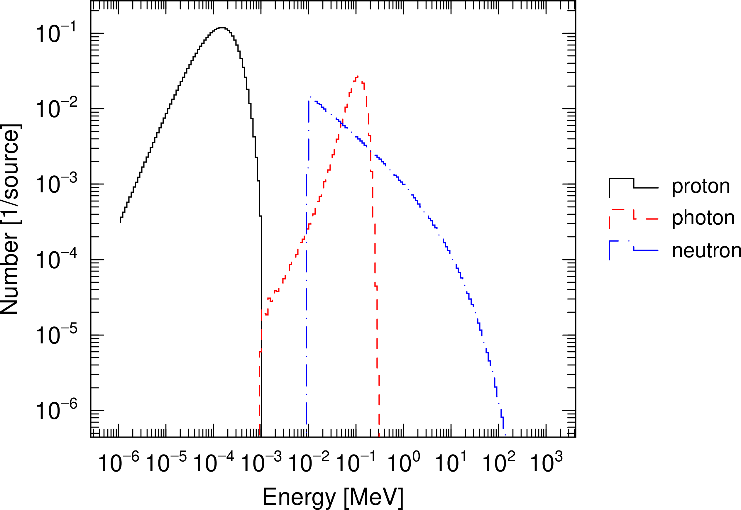
Fig. 5.3.8 Multi-source, energy distribution

The first source has dir=0, that is, 90 degrees. The second has dir=-1, that is, 180 degrees. The third has dir=data and therefore has an angular distribution. Here, a Gaussian distribution centered at 0 degrees is defined by a function. This result is shown below using [t-cross].

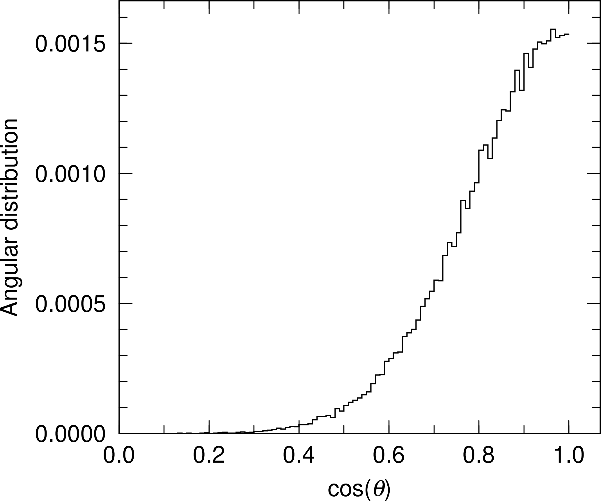
Fig. 5.3.9 Multi-source, angular distribution