2.11. H2: Two dimensional contour graph section
2.11.1. Basic style
H2: section describes three dimensional data as a two dimensional contour graph. Let us start from the following simple example.
List 2.15 • Two dimensional contour graph, example 1
1:  H2: Y = 3.0 TO -3.0 BY -1.0 ; X = -3.0 TO 3.0 BY 1.0 ;
2:   0    0    0    0    0    0    0
3:   0    8    0    2    4    0    0
4:   0    0    1    5    6    2    0
5:   0    2    4   14   15    9    0
6:   0    2    5   23   32   12    0
7:   0    0    3   10   16    8    0
8:   0    0    0    0    0    0    0
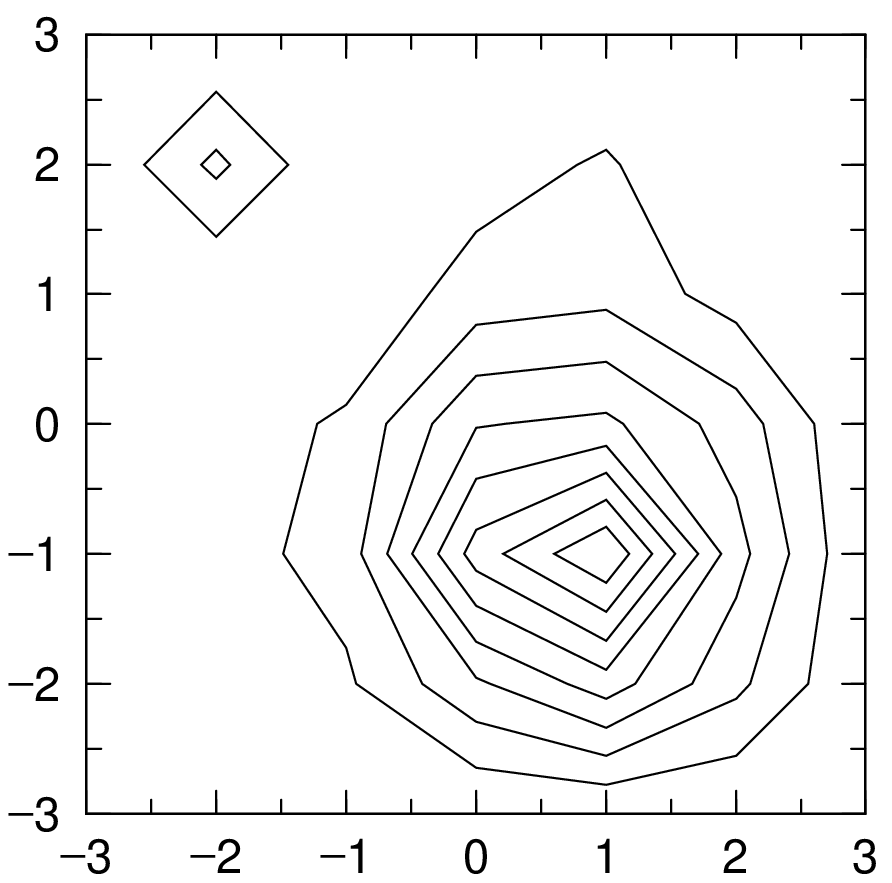
Fig. 2.11 Two dimensional contour graph, example 1
In H2: section, contour lines are described from data on height between two dimensional points given by mesh points with equal width.
In the H2: line, the minimal, maximal and width of mesh points for X and Y axes should be specified. In the above example, the minimum value \(= -3.0\), the maximum value \(= 3.0\), and the width of the meshes \(= 1.0\) for both X and Y axes are defined. The number of the mesh points are automatically determined from these values. The order of this definition determines the order in which the data below this low is read.
H2: Y = 3.0 TO -3.0 BY -1.0 ; X = -3.0 TO 3.0 BY 1.0 ;
This expression comes from the Fortran expression as,
READ(*,*) ( ( DATA(IX,IY), IX = 1,7,1 ), IY = 7,1,-1 )
H2: { Y \(|\) X } = \(r_1\) TO \(r_2\) BY \(r_3\) ; { X \(|\) Y } = \(r_4\) TO \(r_5\) BY \(r_6\) ;
If you want to exchange X axis and Y axis, the order of reading the data has to be exchanged. (In the above Fortran expression, the ordering of IX, IY is exchanged.) The “;” of the end of X axis part and Y axis part is always necessary. The number of the numerical data in a line is free as far as the data sequence is satisfied following the above expression.
2.11.2. Parameters for the contour graph
The number of contour lines and the height, the color, the type of lines, the width and the spline of the contour lines can be changed in the parameter section P:.
parameters |
explanation |
|---|---|
|
Set the number of contour lines as \(i\). The default is 8. |
|
Specify the contour-line heights with \(r_1, r_2, ...\). The number and order of these values are arbitrary. If omitted, the height range is divided into 8 equal parts and 8 contour lines are drawn. |
|
|
|
specify each contour color and grayscale by \(c_1, c_2, c_3, ...\) [2]. These suffix numbers of \(c_n\) correspond to those of |
|
Automatically set the contour colors. |
|
Specify each contour line type with \(L, M, D, ...\). The suffix order corresponds to the contour lines specified by |
|
Specify the colors of the maximum and minimum contour line. |
|
Default is Red(r) and Blue(b). |
|
The interval of the contours is divided equally in linear scale (default). |
|
The interval of the contours is divided equally in logarithmic scale. |
These parameters are valid only without |
|
|
Specify the thickness of line. Default is \(id = 4\) in unit of \(1/300\) inch. |
|
Spline the contour lines by 4 interpolation points (default). If you want to increase the interpolation points, set the number of the points \(n\) such as |
|
Spline the mesh data by Gauss smearing with considering the nearest neighbor mesh (default). If you want to increase the number of neighbor meshes, set the number of neighbors \(n\) such as |
|
Check the numerical values in the two-dimensional data. (default) |
|
Do not check the numerical values in the two-dimensional data. |
By the same input as in example 1 when the IPD2 and COLS are specified, the result is shown below.
List 2.16 • Two dimensional contour graph, example 2
1:  P: IPD2 COLS
2:  H2: Y = 3.0 TO -3.0 BY -1.0 ; X = -3.0 TO 3.0 BY 1.0 ;
3:   0    0    0    0    0    0    0
4:   0    8    0    2    4    0    0
5:   0    0    1    5    6    2    0
6:   0    2    4   14   15    9    0
7:   0    2    5   23   32   12    0
8:   0    0    3   10   16    8    0
9:   0    0    0    0    0    0    0
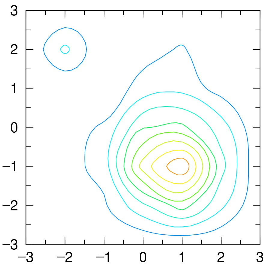
Fig. 2.12 Two dimensional contour graph, example 2