2.10. H:   One dimensional graph section

2.10.1. Basic style

2.10.1.1. Basic style 1

The main role of H: section is a definition of ordering of the data written below. We show again the part of input data of tutorial example 1 below.

List 2.3 • Basic style 1

1:  H: X     Y
2:     0.5   10
3:     3     40

In this case, the line of H: declares that there are two columns and that the first one is X column, and the second one is Y column. ANGEL can judge how many lines are included in this section. The number of the data is only restricted by your memory. If you need more memory, you should change mdas parameter in angel00.in file.

2.10.1.2. Basic style 2

In below example, there is one X column but there are four Y columns. X column should be only one in a H: section, but you can define Y column up to 30.

List 2.4 • Basic style 2

1:  H:  X     Y1     Y2     Y3      Y4
2:      0.5   10      1     .4    10.5
3:      3     50      2     .5    13.3
4:      5     30      3     .6    12.3

Using this input file, four lines are drawn as a function of the same x values. In the above input, the digits following Y in Y1  Y2  Y3  Y4 may be omitted. These are necessary for the error column and column function discussed later. For this case, Y  Y  Y  Y is enough. The ordering of the X and Y columns is free. You can therefore easily exchange the x and y values by writing Y  X instead of X  Y in the H: section without changing the data ordering.

2.10.1.3. Basic style 3

To skip data columns, change the character that specifies the meaning of the column. For example, to skip the second and third columns in the above input data, write N or NY instead of Y. However, if a Y value is missing for a certain X row, this results in an error, as shown below.

List 2.5 • Basic style 3

1:  H:   X    Y1    NY2     N3     Y4
2:      0.5   10      1     .4    10.5
3:      3     50      2           13.3
4:      5     30      3     .6    12.3

This is an error. A Y value must exist for every X row. Data with missing Y values must be placed in a separate H: section.

We summarize the basic parameters of H: section in the following.

Table 2.8 Column parameter

parameter	explanation	remark
X	X column	Only one column without suffix.
Y	Y column	Maximum 30 columns; a numeric suffix may be added.
DX	X error column	A numeric suffix may be added.
D	Y error column	A numeric suffix may be added.
N, NX, NY, ND, NDX	skip column	A numeric suffix may be added except to NX, NDX.

2.10.2. Factor

You can multiply, divide, sum or subtract a constant from the data in X, Y, D, DX column. For an example,

List 2.6 • Example of factor

1:  H:   X   Y*1.0E+03-500.0
2:     0.5   10
3:     3     40

This example multiplies 1000 on the Y value and subtracts 500. These values after calculation are plotted in a graph. This factor function is also available for X column. The format of this factor function is

[ * \(r_1\) ] [ { \(|\) / } \(r_2\) ] [ { + \(|\) - } \(r_3\) ]

where [   ] means optional, { \(A\) \(|\) \(B\) } denotes that you should choose \(A\) or \(B\), and \(r_1, r_2, r_3\) are positive numbers. To use a negative number, enclose it in (  ), as in (\(-r_1\)), (\(-r_2\)), or (\(-r_3\)). User-defined constants and mathematical expressions cannot be used as \(r_1, r_2, r_3\). Therefore, complicated mathematical expressions cannot be expressed with this factor function. In such cases, use the column function explained later. The points to note about the factor function are

• Ordering : [power], [multiply \(|\) divide], [sum \(|\) subtract]

• first and intermediate blank is not allowed

• (   ) should be used for negative number

2.10.3. Legend

As shown in Tutorial example 2, you can easily draw legend of lines. It is very convenient when you plot several lines in one graph. As an example,

List 2.7 • Example of legend

1:  H:  X   Y(Histogram),DH0
2:      0.0    0
3:      0.5   10
4:      1.5   20

The strings inside (   ) just after Y or Y3 and before a comma are shown with the symbol and/or line type at the middle of right handside of graph frame. The ordering of the legends is that of appearance of input file. The position of the legend can be moved by parameter. The remarks of the format of legend are

• draw parentheses in (    ) as \(   \)

• no blank before and after (    )

And the blank inside (    ) is no matter, and also the ordering between factor and legend is free.

The parameters which change scale, position and color are listed in the following table.

2.10.3.1. Legend parameters

Table 2.9 Legend parameter

parameters	explanation
LEGN	Show legend (default).
NOLG	Do not show legend.
LEGX( \(x\) )	Set the left hand side of legend to be \(x\) in X axis.
LEGY( \(y\) )	Set the top of legend to be \(y\) in Y axis.
LEGS( \(s\) )	Change scale of legend by \(s\) (D=1).
CLLG( \(c\) )	Change color of legend to \(c\) [1] (D=e).
LBOX( \(boxname\) )	Show frame around by \(boxname\) [2].
LBCB( \(cb\) )	Change color of background of box to \(cb\) (D=w).
LBCL( \(cl\) )	Change color of frame of box to \(cl\) (D=e).
LBCS( \(cs\) )	Change color of shadow of box to \(cs\) (D=e).

[1]

color definition is explained in line parameter section.

[2]

\(boxname\) definition is explained in BOX: section.

2.10.4. Line parameters

You can specify line type, symbol, spline, histogram, and the other line descriptions by parameters after a comma in Y part.

In the example of Tutorial example 2, DH0 of H:  X   Y(Histogram),DH0 is line parameter. DH0 means that line type is dashed line with histogram without symbol.

2.10.4.1. Line type

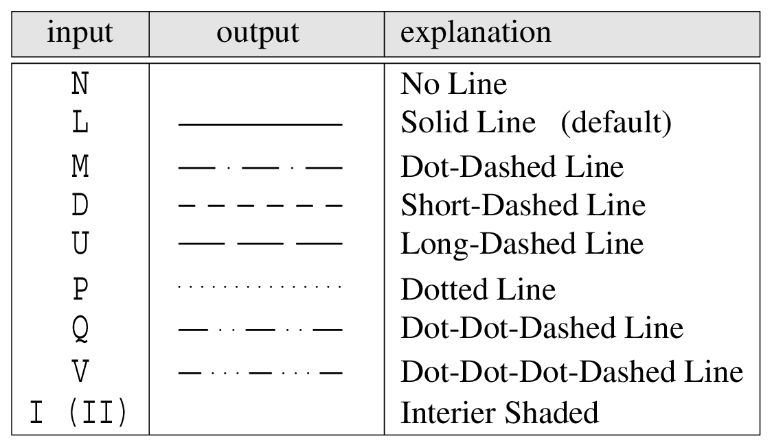
There are nine types of lines which is specified by alphabet symbol as

Table 2.10 Line type

Interior shaded I and II paints the region within the line with defined color. You can change the color or gray scale by color parameter. The region is clipped within the graph frame by I, but not clipped by II.

2.10.4.2. Length of pattern of line type

You can change the length of pattern of line type by LPTL in parameters section.

Table 2.11 Length of pattern parameter

parameter	explanation
LPTL( \(r\) )	Change unit length to \(r\) (D=1).

The unit of length is the default length of the pattern.

2.10.4.3. Line thickness

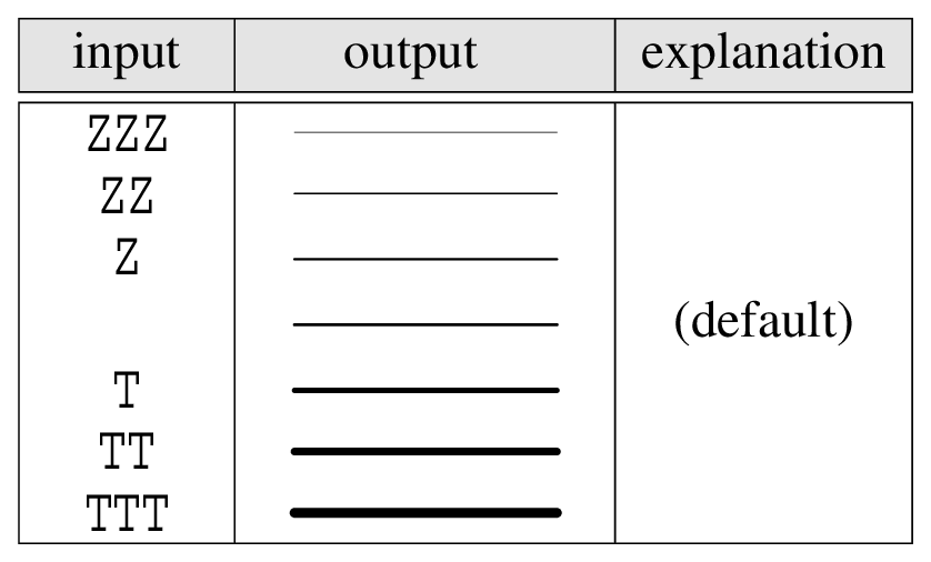
You can change thickness of lines by Z and T as

Table 2.12 Line thickness

2.10.4.4. Spline

In default, ANGEL connects two data points by straight line. If you add line parameter ’S’, ANGEL connects the data with spline line as shown in Tutorial example 2.

ANGEL interpolates four points between two data if you specify ’S’. The number of points for interpolation is changed by adding number after ’S’ as

S[ \(n\) ]

where \(n\) is the number of points for interpolation, which should be described in [  ].

2.10.4.5. Symbol

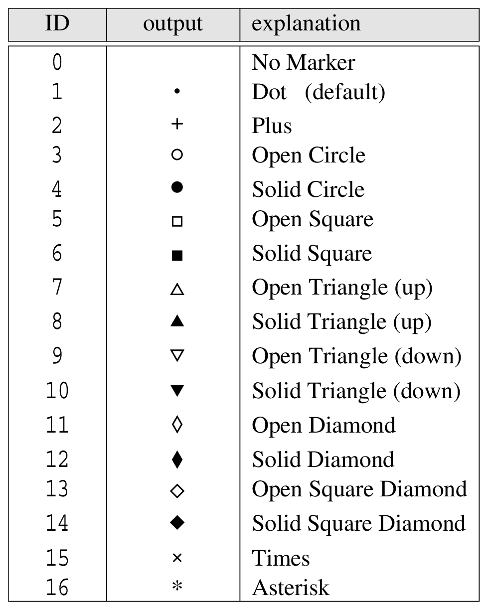
There are 16 kinds of symbols drawn on the data points, as follows.

Table 2.13 Symbol

2.10.4.6. Option of Symbol

The odd-numbered symbols from 3 to 13 are hollow. Their interiors are not transparent, as shown by the Spline line in Tutorial example 2, but are filled with white.

If you want to change the hollow part to be transparent, you add 20 to ID number of these symbols. When you change the color of these symbols, the hollow part keeps white. If you want to change the color of the hollow part, you should write as 5[R]. You can specify the color of the hollow part by color definition within [  ] just after symbol ID.

Thickness of symbols is proportional to the thickness of lines. You can also change the thickness of symbols separately in parameter section as

Table 2.14 Symbol parameter

parameter	explanation
SYBW( \(r\) )	Change thickness of symbol to be \(r\) (D=1).

This parameter affects all symbols.

2.10.4.7. Size of symbol

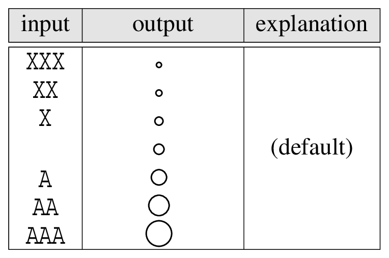
You can change the size of symbol by X and A as

Table 2.15 Size of symbol

2.10.4.8. Grayscale

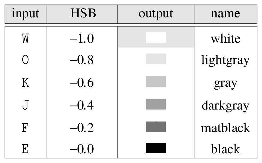
The grayscale is defined by alphabet symbols as in the next table. There are 6 degrees of grayscale. If you use C[\(f\)] description mentioned later, you can define the grayscale continuously.

Table 2.16 Grayscale

2.10.4.9. Color

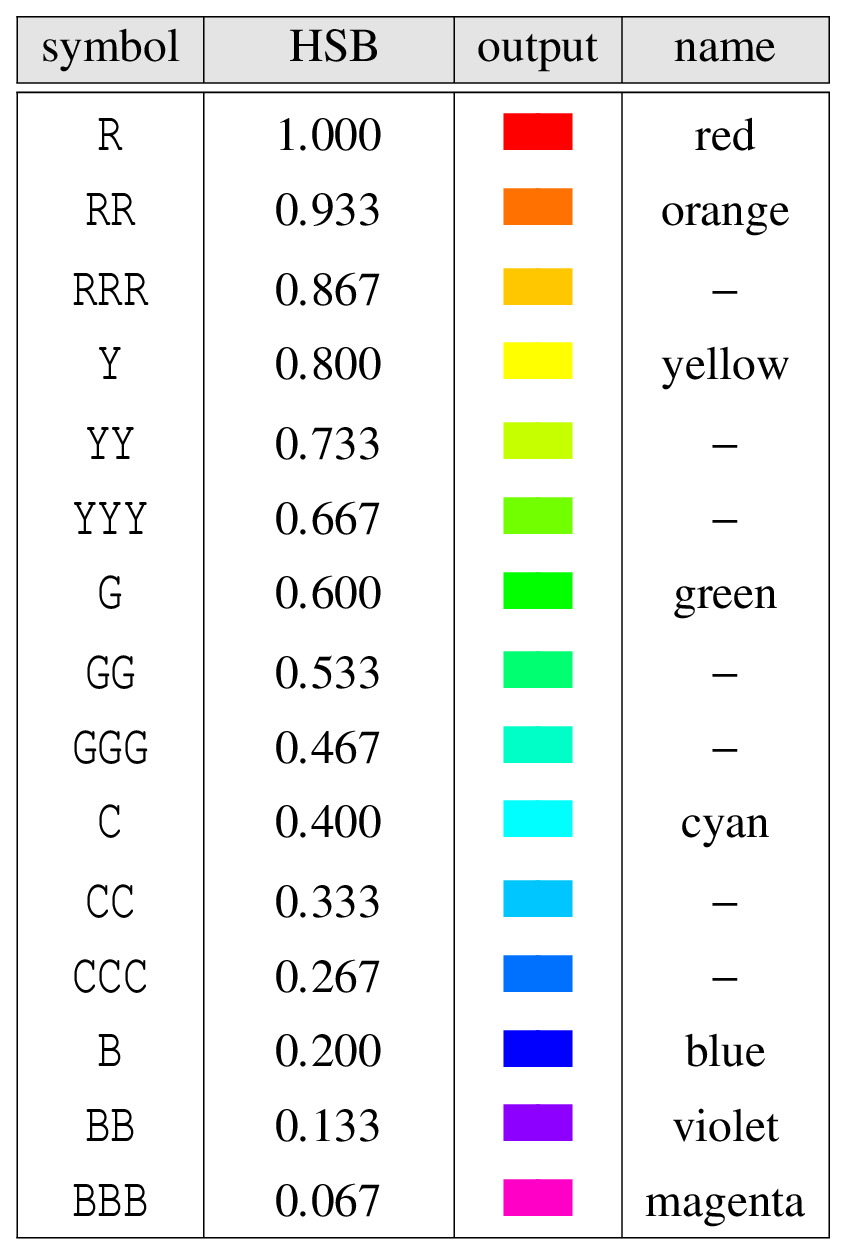
The colors of lines and symbols are defined by the following symbols in the line-parameter part. The basic colors consist of five colors, and intermediate colors are specified by a pair or triplet of symbols. Using the C[\(f\)] color notation described later, you can specify colors continuously by HSB (Hue, Saturation, Brightness) values or by name. The symbols define only the Hue value; Saturation and Brightness are both one in this case.

Table 2.17 Color defined by symbol

2.10.4.10. HSB or name definition for grayscale and color

You can define the grayscale or color by HSB value or name as

C[ \(H(\)Hue\() \, S(\)Saturation\() \, B(\)Brightness\()\) | name ]

Although C is used as the color symbol for Cyan, C followed immediately by [  ] defines a color or grayscale by HSB values or by name. A negative \(H(\)Hue\()\) specifies grayscale; in this case, \(S(\)Saturation\()\) and \(B(\)Brightness\()\) have no meaning and may be omitted. For color, \(H(\)Hue\()\) must be positive, and \(H(\)Hue\()\), \(S(\)Saturation\()\), and \(B(\)Brightness\()\) must be between zero and one. If \(S(\)Saturation\()\) and \(B(\)Brightness\()\) are omitted, one is assumed for each. The next page shows a color map with varying HSB values.

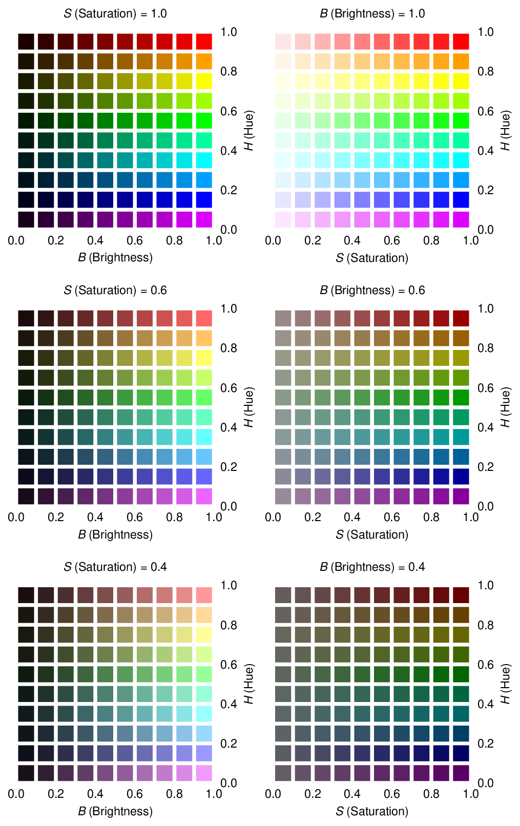
Fig. 2.3 Color map

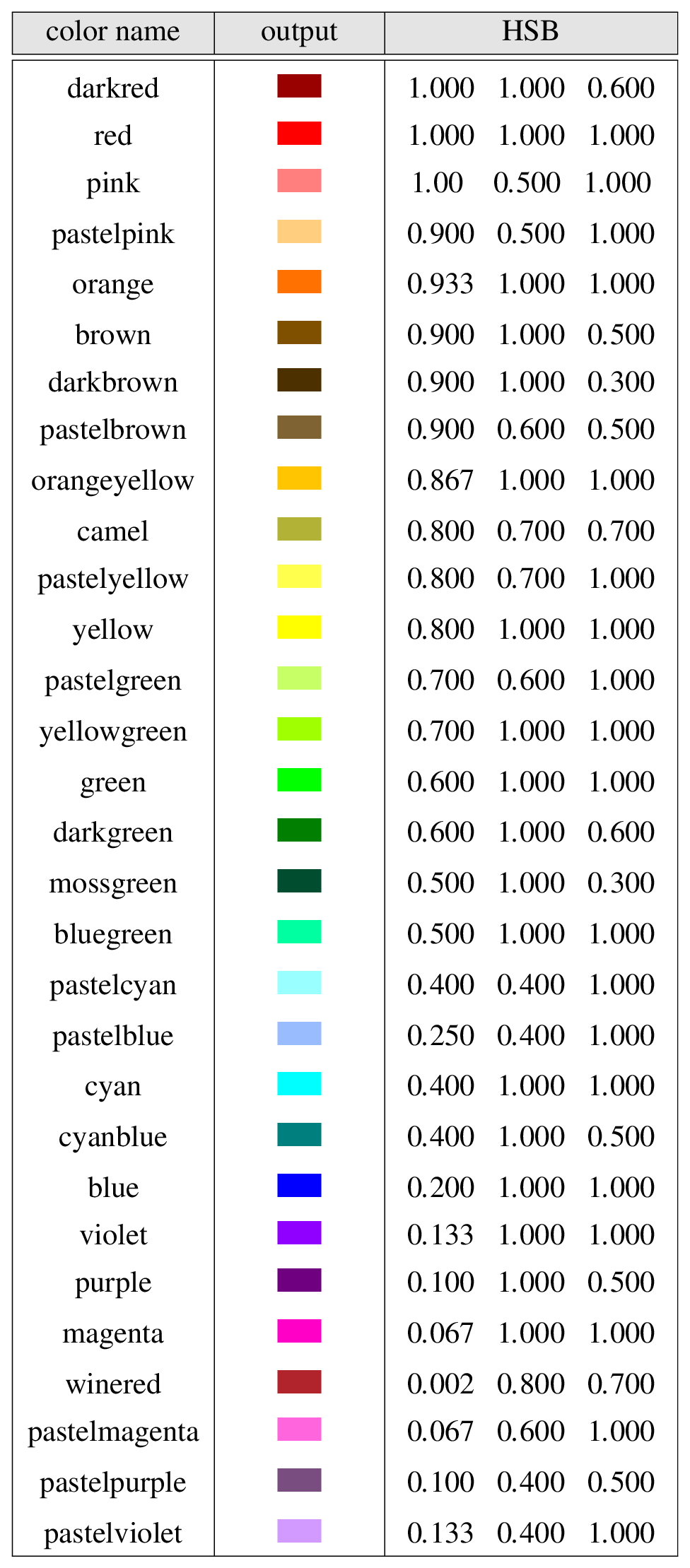
Fig. 2.4 Color defined by color name or HSB

2.10.4.11. Histogram

You can draw histogram by adding ’H’ in line parameter as shown in Tutorial example 2. In histogram, you have to choose the relationship between data points and corners of histogram. In default, the y value of a data point keeps the value up to the next x point. Thus the data point is shown by the left corner of histogram as

List 2.8 • Example of histogram 1

1:  H:  X   Y(ex1 H),LH6
2:      0.0    0
3:      0.5   10
4:      1.5   20
5:      2.5   35
6:      3.5   30
7:      4.5   45
8:      5.5   70
9:      6.5    0

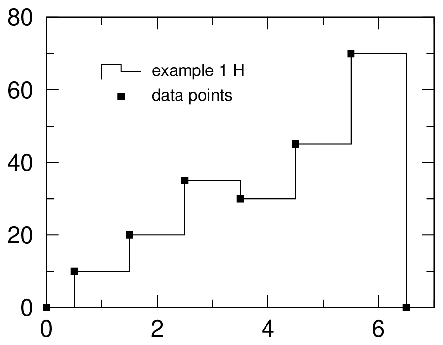
Fig. 2.5 Example of histogram 1

If you write ’HH’ or ’HHH’ instead of ’H’ in line parameter, you can change the corner of histogram.

Fig. 2.6 Example of histogram 2

Fig. 2.7 Example of histogram 3

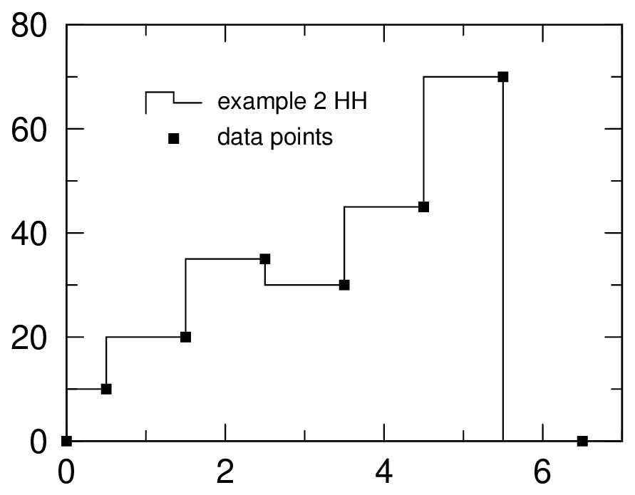
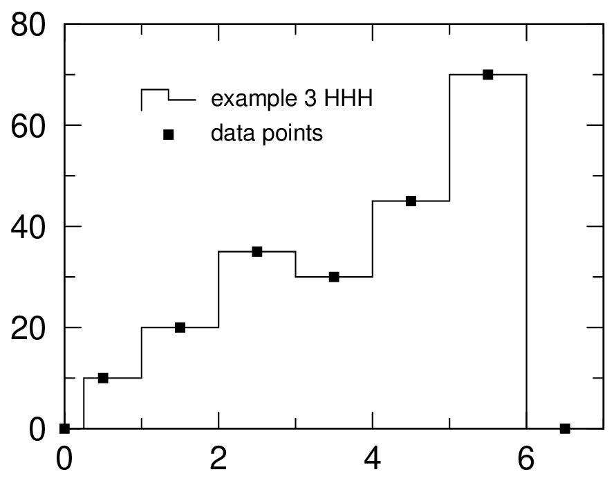
As shown in above graph, you can choose the relation between the data points and the corner of histogram.

2.10.5. Summary and remark in Y column format

Here we summarize the format of Y column and remark some points.

• Y[ID digit][(legend strings)][factor],

  [line type][thickness][symbol ][size of symbol][spline][histogram]

• any blank is not allowed except in legend strings.

2.10.6. Error bar

The column of error bar data is specified by ’D’ or ’DX’ in H: section. The values of error should be absolute values. If the values of error are % of the y-value or relative value, you can use column function mentioned later.

2.10.6.1. Error bar for Y value

The basic style of error bar for y values is that you prepare ’D’ column just after ’Y’ column.

List 2.9 • Basic style of error bar 1

1:  H:  X     Y    D
2:      1    10    3
3:      3    50    4

In this case, \(\pm\)3 error bar in y direction is shown at the point (1,10).

If you want to draw error bars which values are different between upside and downside, you should prepare two ’D’ column like D+  D- after y column by adding + and -.

List 2.10 • Basic style of error bar 2

1:  H:  X     Y    D+    D-
2:      1    10    3     2
3:      3    50    4     3

In this case, 3 error bar for + side of y direction, 2 error bars for - side of y direction are shown at the point (1,10). If you want to draw both side error bar by one error column, you should write D+- for the column, which is equivalent to default style of D

If there are some ’Y’ columns and also ’D’ column in a H: section, ’D’ column just after ’Y’ column is the error bar for the y values in default. In order to change the ordering on column more freely, you can put ID digit after ’Y’ and ’D’ like

List 2.11 • Basic style of error bar 3

1:  H:  X    Y1    Y2      D2      D1
2:      1    10    1.1    0.3      3
3:      3    50    1.3    0.4      4

In this case, \(\pm\)3 error bar is shown at the point (1,10) of ’Y1’ column, \(\pm\)0.3 error bar is at (1,1.1) of ’Y2’ column. ID digit can be used from 1 to 10, and the ordering is free. If you want to put the ID digit on one ’Y’ column, you should put ID digit on all other ’Y’ and ’D’ column identification.

You can also use factor for error bar column as in y column.

Here, we summarize the above error bar for Y column as

• D[ID digit][+][-][factor]

• [+][-] should be prior to [factor]

2.10.6.2. Error bar for X value

Error bar column can be specified by ’DX’. The basic format of ’DX’ is almost the same as that for Y column. In the following, we summarize different points from the error bar format for Y column as,

• ID digit cannot be used.

• If there are some Y columns, the same error bars for x direction are shown in each point of different Y columns.

Therefore if you want to draw the different error bar for X value, you have to describe each Y value in different H: section with different error bar for X values.

2.10.7. Column function

By using ’factor’, you can change the column values by simple mathematical expression with some constants. If you change them in more complicated equation, or if you want to use the value of the other column in addition to constants, you can use ’column function’. The basic style of the column function is

\(\langle\) column parameters \(\rangle\langle\) ID digit \(\rangle\)=[ equation  ]

where column parameters denote X, Y, DX, D, NY, ND listed in Table 2.8, and ID digit is necessary for Y, D, NY, ND. Any blank is not allowed before and after =. But you can use some blanks in equation within [   ]. In the equation, you can use real number, user definition constants, intrinsic constant (pi, ran), intrinsic function, Fortran equation, and functional fit, self-running variable, which are introduced in the following sections, and X and Y column values specified by the column parameters.

A simple example is shown below,

List 2.12 • Example of column function

1:  H:  X     Y1,D6   NY2   DY1=[Y1*Y2/100]
2:      0.0    0.0     0.0
3:      1.0    0.4    50.0
4:      2.0    1.5    30.0
5:      3.0    2.5    20.0
6:      4.0    4.1    10.0

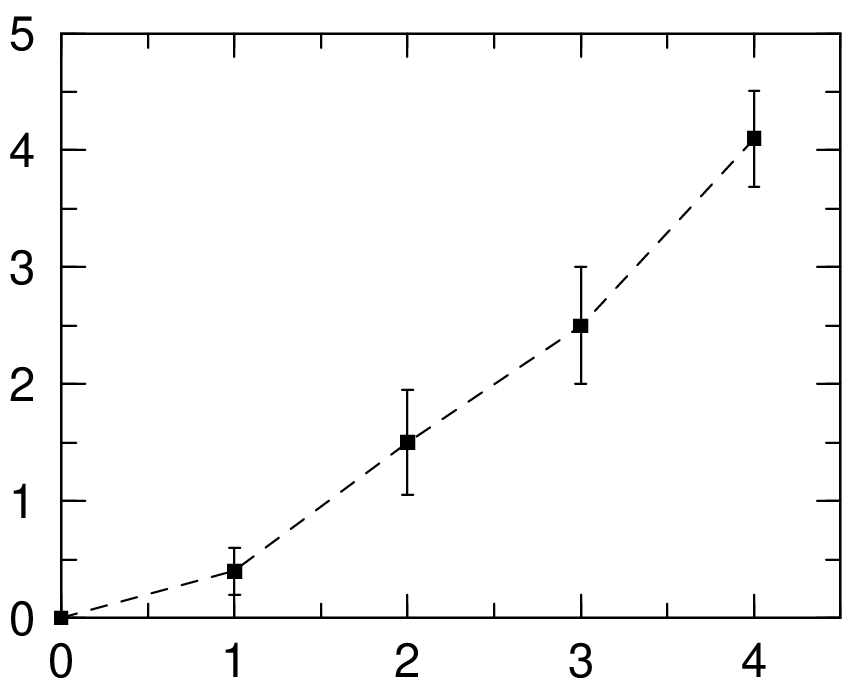
Fig. 2.8 Example of column function

In this example, the first column is X value, the second Y value, and the third column is the relative error of Y value as %. You cannot draw the error bar by this error value, since the values of error should be given by absolute value in ANGEL . You have to transform the relative values of error to the absolute values using the column function. You first change the column parameter of the third column to ’NY2’, and you define the fourth column by column function as DY1=[Y1*Y2/100]. The graph of this input is shown here. In the column function, you can only use the value of X and Y column. We define the column parameter of the third column as ’NY2’ not as ’ND1’. We summarize the rule of the column function as following,

• \(\langle\) column parameters \(\rangle\langle\) ID digit \(\rangle\)=[ equation  ]

• any blank is not allowed except in [   ]

• column function should be prior to legend and [+][-] of error

• do not use ’N’ of column parameters in equation; (NY2 \(\to\) Y2)

2.10.8. Self-running variable V

You can plot various values obtained by the column function from the other column values. When you want to plot analytic function of x values, you have to write down x-column values. In this case, you can define self-running variables ’V’ for the x column values. The format of self-running variable is

V=[ \(r_1\), \(r_2\), \(n\) ]

where any blank is not allowed except in [   ]. In this format, \(r_1\) and \(r_2\) are the minimum and maximum values and \(n\) is number of value points. The self-running variable gives \(n\) points from \(r_1\) to \(r_2\) divided equally by \(n - 1\) groups. You can use user definition constants and mathematical expressions for \(r_1\) and \(r_2\).

By this self-running variable and column function, you can plot any analytical function on a graph without explicit x column values.

We show an example of the self-running variable and column function in the following.

List 2.13 • Example of self-running variable

1:  H:  V=[0,2*pi,100] X=[V/pi] Y=[0.8*sin(V)],L0
2:  H:  V=[0,2*pi,100] X=[1.0+0.5*cos(V)] Y=[0.5*sin(V)],D0

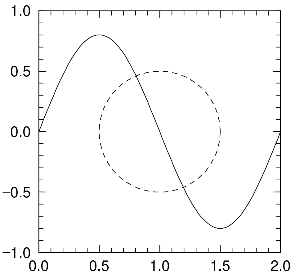
Fig. 2.9 Example of self-running variable

In the above example, the self-running variable V prepares 100 values from 0 to 2\(\pi\). In the first H: section, X is defined by V/\(\pi\) and Y is a sine function of X. In the second H: section, X and Y are defined by the cosine and sine function of V. This is a circle with (1.0,0) center and 0.5 radius.

Here, we summarize the format of self-running variables.

• V=[ \(r_1\), \(r_2\), \(n\) ]

• any blank is not allowed except in [   ]

• user definition constant and mathematical expression can be used for \(r_1\) and \(r_2\).

2.10.9. Fitting function

Using ANGEL , you can fit the data points (x,y) by an analytical function. We use the least squares methods for fitting the data with considering the error bar if it exists.

The basic style of the fitting function is similar to the style of the column function and is given by

\(\langle\) column parameter 1 \(\rangle\langle\) ID digit \(\rangle\)=F{ \(\langle\) column parameter 2 \(\rangle\) }[ analytical function ( An ) ]

where column parameter 1 is a column for the fitting function with Y, NY and column parameter 2 is a Y column for fitting data. Any blanks are not allowed before and after =F.

But you can use blanks within {   } and [   ]. In the fitting function, you can use real number, user definition constants, intrinsic constant (pi, ran), intrinsic function, and any equation in Fortran style, and X and Y column values specified by the column parameters in the same H: section.

For the coefficients in the fitting function, you should use the coefficient variables A.

The suffixes of A are from A1 to A99. These coefficient variables can be used in the other places after the fitting function like user definition constant.

Let see a simple example below.

List 2.14 • Example of fitting function

1:  H:  X     Y1,D6    D1    NY2=F{ Y1 }[ A1 * X**2 ]
2:      0.0    0.0     0.0
3:      1.0    0.4     0.2
4:      2.0    1.5     0.45
5:      3.0    2.5     0.5
6:      4.0    4.1     0.41
7:  H: V=[0,4.5,100] X=[ V ] Y=[ A1 * X**2 ],L0TT

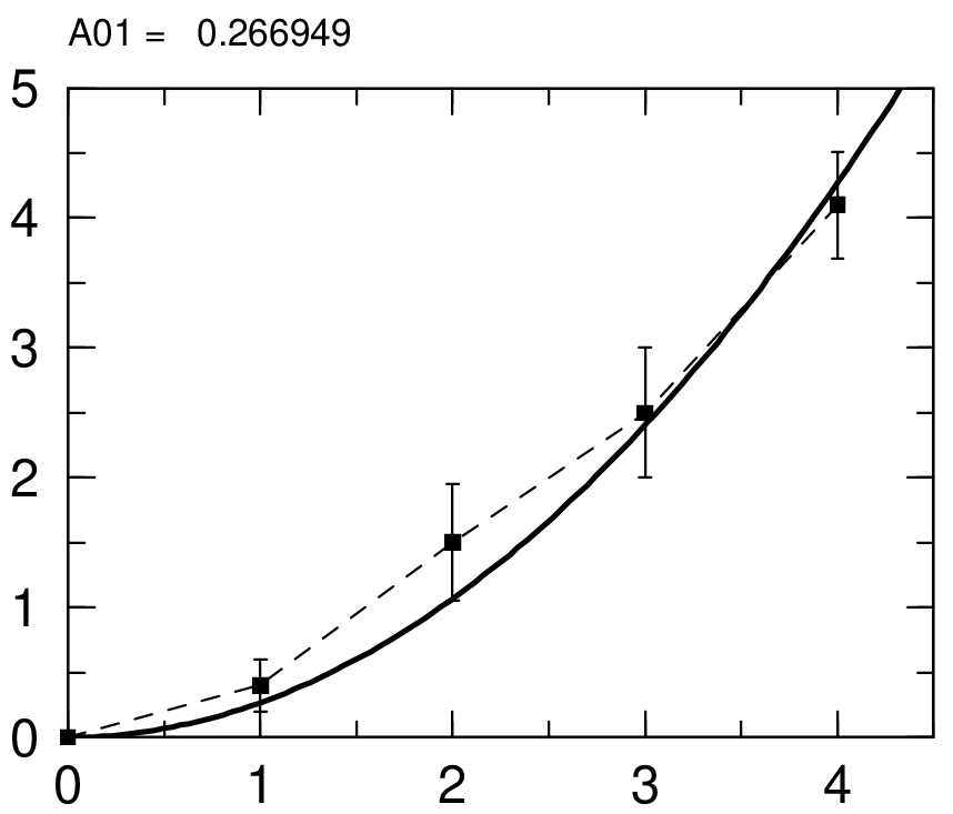
Fig. 2.10 Example of fitting function

In this example, X and Y1 columns are the same as in the example of column function.

The error column should be converted to the absolute values.

We fitted these data points by the function of \(y = a_1 x^2\). After the ANGEL processing, the values of A1 and the squares of the error of fitting are shown in the normal output.

Since ANGEL uses the Metropolis method for fitting, the results differ a little in each processing. If the correlation between the data and the fitting function is not enough, the coefficients are not converged and give us almost zero values in each processing.

As in the above example, if we plot the fitting function in the same H: section, the X values of the fitting function are the same points as the data. In this case, we cannot obtain smooth shape of the fitting function. So we have not plotted the fitting function in the same H: section, we specified NY2, but we have plotted it in the next H: section by using the self-running variables and the coefficient variables in the above example to get smooth shape of the fitting function.

These coefficients obtained from fitting the function to data can be shown in the figure.

In default, these are shown at the left corner above the figure frame as in the previous example. When changing the position, scale and the other format, you can use the following parameters in the parameter section P:.

2.10.9.1. Parameters for the fitting function

Table 2.18 Parameters for the fitting function

parameters	explanation
PARA	Show the coefficients of the fitting function.
NOPA	Do not show the coefficients of the fitting function (default).
PARX( \(x\) )	Set x-position of the coefficients as \(x\).
PARY( \(y\) )	Set y-position of the coefficients as \(y\).
PARS( \(s\) )	Change the scale of the expression as \(s\) (D=1).
CLPA( \(c\) )	Change the character color to \(c\) [3] (D=e).
PBOX( \(boxname\) )	Enclose the expression by the box of \(boxname\) [4].
PBCB( \(cb\) )	Change the color of the background of the box as \(cb\) (D=w).
PBCL( \(cl\) )	Change the color of the frame of the box as \(cl\) (D=e).
PBCS( \(cs\) )	Change the color of the shadow of the box as \(cs\) (D=e).

[3]

Definition of the color is shown in the line parameters section

[4]

Definition of \(boxname\) is shown in BOX: section.

Here we summarize the fitting function.

• \(\langle\) Column parameter 1 \(\rangle\langle\) ID digid \(\rangle\)=F{ \(\langle\) Column parameter 2 \(\rangle\) }[ fitting function( An ) ]

• any blank is not allowed except in {   }, [   ]

• do not use “N” for the column parameter 2 (NY2 \(\to\) Y2)

• do not use “N” for the fitting function (NY2 \(\to\) Y2)