4.13. 例題: 3-ステップ 崩壊線量計算 (reg/xyz メッシュ)
本例題では、放射化生成物の時間依存崩壊スペクトルを線源とする輸送計算を、DCHAINとPHITSを組み合わせて実行する方法を示す。放射化したターゲットを含む室内の周辺線量当量率\(\dot{H}^*(10)\)の空間分布を評価する。この手法は、照射スケジュール、冷却時間、材料組成、遮蔽構造が空間線量分布へ与える影響など、さまざまな実体系の線量評価へ応用できる。計算は次の3段階で行う。
イオンビームや中性子源などの照射線源を有効にし、[T-Dchain]を設定したPHITS計算を実行して、中性子フラックスと高エネルギー核反応による核種生成率を求める。
[T-Dchain]が生成したファイルをDCHAINへ入力し、放射化、核種インベントリの時間変化、崩壊放射線スペクトルを計算する。
DCHAINが
*.phtファイルへ出力した崩壊放射線の[Source]セクションをPHITSへ挿入し、元の照射線源を無効にして、必要なタリーを設定したPHITS計算を再実行する。運転中の評価では、必要に応じて元の照射線源も有効にする。
本例題は前節の計算と似ているが、ターゲットを円柱から直方体へ変更し、周囲に室内体系を追加している。
直径1 cmのペンシル状250 MeV陽子ビームを、タングステン、水、鉄の3区間で構成される直方体ターゲットへ入射する。ターゲットの側面と後端はベリリウムで覆われている。ビーム電流100 nAで10分間照射した後、合計50分間冷却する。
評価対象は、照射終了5分後にターゲットのタングステン部の放射化によって生じる、室内の周辺線量当量率\(\dot{H}^*(10)\)分布である。ターゲットと室内の体系を 図 4.13.1 から 図 4.13.2 に示す。ビームは\(z=-10\)cmから\(+z\)方向へ進み、最初にタングステン表面へ入射する。
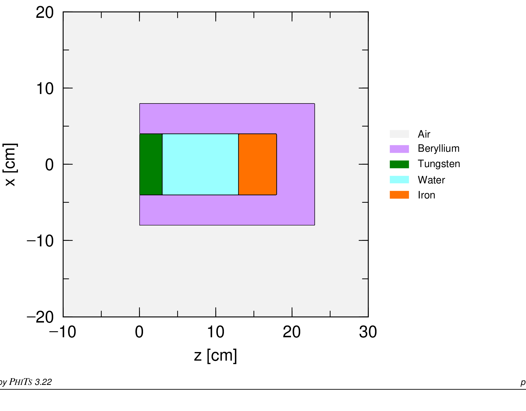
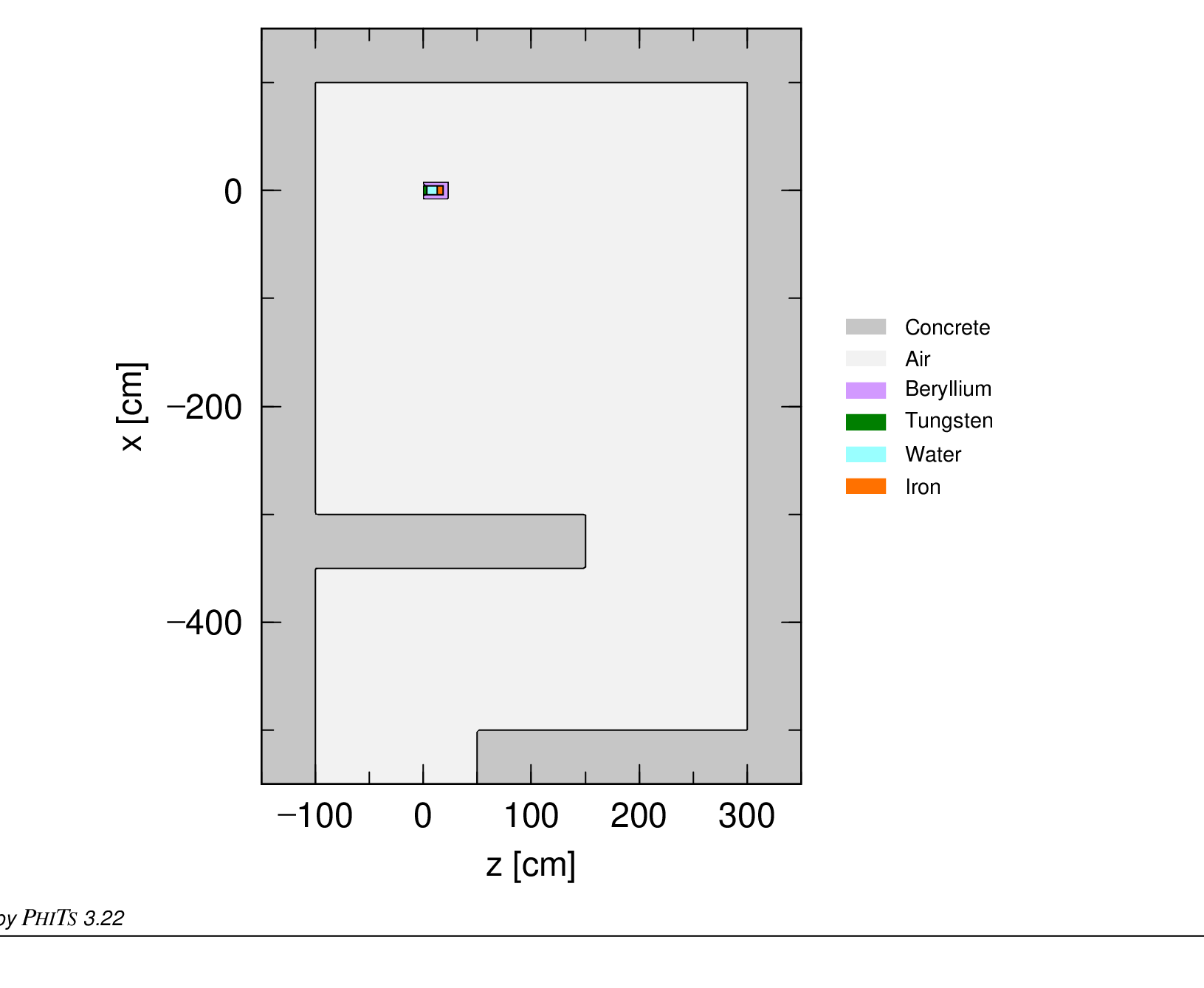
本例題で使用し、段階ごとに変更するPHITS入力ファイルは<PHITS-install>/dchain-sp/sample/3-step_dose_xyz/phits_3-step.inpにあり、付録6.3 にも掲載している。入力には、後で有効にするコメント行や無効化されたセクションが含まれる。主な箇所は、[Source]セクション直前のファイル挿入行、[Cell]セクションの室内空気・コンクリート領域、最後の[T-Track]タリーである。
2つの[T-Gshow]タリーは 図 4.13.1 から 図 4.13.2 の作成に使用した。本例題で示す出力は、すべてPHITSまたはDCHAINによって自動生成される。また、[T-Dchain]におけるxyzメッシュの使用方法と、regメッシュとの差が結果へ与える影響も説明する。
[Title]
Dose from 250MeV protons activating W/H2O/Fe block surrounded in Be

[Parameters]
 icntl    =           0     # (D=0) 3:ECH 5:NOR 6:SRC 7,8:GSH 11:DSH 12:DUMP
 maxcas   =      100000     # (D=10) number of particles per one batch
 maxbch   =          10     # (D=10) number of batches
 file(1)  = c:/phits        # (D=c:/phits) PHITS install folder name
$  required options for DCHAIN
 file(21) = c:/phits/dchain-sp/data # (D=c:/phits/dchain-sp/data) DCHAIN data folder
 jmout    =           1     # (D=0) Density echo, 0:input, 1:number density
 e-mode   =           0     # (D=0) Event generator mode is not recommended for DCHAIN
 igamma   =           3     # (D=2) 0:No, 1:Old, 2:EBITEM, 3:EBITEM+Isomer

$ Photon source from DCHAIN output
infl:{W_xyz_target_gamma_t3.pht}
$ This needs to come before the "off" source section or it will be skipped.

[Source] off
   s-type =   1             # mono-energetic axial source
     proj =  proton         # kind of incident particle
       e0 =   250.00        # energy of beam [MeV/u]
       r0 =   0.5000        # radius [cm]
       x0 =   0.0000        # (D=0.0) center position of x-axis [cm]
       y0 =   0.0000        # (D=0.0) center position of y-axis [cm]
       z0 =  -10.000        # minimum position of z-axis [cm]
       z1 =  -10.000        # maximum position of z-axis [cm]
      dir =   1.0000        # z-direction of beam [cosine]

[Material]
$ Tungsten, Density (g/cm3) = 19.300000
M1      74000  1.000000  $  W
$ Water, Density (g/cm3) = 0.998207 ~= 1.0
M2       1000  0.666657  $  H
         8000  0.333343  $  O
$ Iron, Density (g/cm3) = 7.874000
M3      26000  1.000000  $  Fe
$ Beryllium, Density (g/cm3) = 1.848000
M4       4000  1.000000  $  Be
$ Air (dry, sea level), Density (g/cm3) = 0.001205
M10      6000  0.000150  $  C
         7000  0.784431  $  N
         8000  0.210748  $  O
        18000  0.004671  $  Ar
$  Concrete, Ordinary (NIST), Density (g/cm3) = 2.300
M11      1000  0.305330  $  H
         6000  0.002880  $  C
         8000  0.500407  $  O
        11000  0.009212  $  Na
        12000  0.000725  $  Mg
        13000  0.010298  $  Al
        14000  0.151042  $  Si
        19000  0.003578  $  K
        20000  0.014924  $  Ca
        26000  0.001605  $  Fe

set:c1[3]  $ thickness of W portion
set:c2[10] $ thickness of H2O portion
set:c3[5]  $ thickness of Fe portion
set:c4[5]  $ thickness of Be back end
set:c5[4]  $ half side length of inner rectangular prism
set:c6[8]  $ half side length of outer rectangular prism

[Surface]
$ Target components
1 rpp -c5 c5 -c5 c5 0     c1            $ W portion
2 rpp -c5 c5 -c5 c5 c1    c1+c2         $ H2O portion
3 rpp -c5 c5 -c5 c5 c1+c2 c1+c2+c3      $ Fe portion
4 rpp -c5 c5 -c5 c5 0     c1+c2+c3      $ Be inner border
5 rpp -c6 c6 -c6 c6 0     c1+c2+c3+c4   $ Be outer border

$ Room structure
15 rpp -350 -300  -100  200  -100  150  $ inside shield
16 rpp -550 -500  -100  200  -100   50  $ doorway
20 rpp -500  100  -100  200  -100  300  $ inner wall
21 rpp -550  150  -150  250  -150  350  $ outer wall

[Cell]
$ Target
1   1 -19.3    -1               $ W
2   2 -1.0     -2               $ H20
3   3 -7.874   -3               $ Fe
4   4 -1.848    4 -5            $ Be

$ Room (void)
$ 10  0          -16:(5 -20 15)   $ room + doorway air
$ 11  0          -15:(20 -21 #10) $ outer + maze concrete walls
$ Room (with materials)
10 10 -0.0012  -16:(5 -20 15)   $ room + doorway air
11 11 -2.3     -15:(20 -21 #10) $ outer + maze concrete walls

99 -1  21                       $ outer void / particle graveyard

[Volume]   $ required section for DCHAIN
   reg   vol
     1   c1*(2*c5)**2
     2   c2*(2*c5)**2
     3   c3*(2*c5)**2
     4   ((c1+c2+c3+c4)*(2*c6)**2)-((c1+c2+c3)*(2*c5)**2)

[Mat Name Color]
   mat     name     size          color
     0     void     1.00     lightgray
     1    Tungsten  1.00     darkgreen
     2    Water     1.00     pastelcyan
     3    Iron      1.00     orange
     4    Beryllium 1.00     pastelviolet
    10    Air       1.00     {-0.9}
    11    Concrete  1.00     gray

$ Beam settings to be used in [T-Dchain] tallies
set:c11[100.0]                           $ beam current (nA)
set:c12[ c11 * 1.0e-9 / (1.602177e-19) ] $ beam power (source/sec)

[T-DCHAIN] off
  title = W target (reg)
  mesh = reg
  reg = 1
  file = W_reg_target.in     # file name of dchain input file
  timeevo =    2             # time evolution / irradiation schedule
    10.0 m 1.0
    50.0 m 0.0
  outtime =    4             # output times
    10.0 m
    -1 m
    -5 m
    -50 m
  amp = c12                  # (D=1.0) Source Intensity(source/sec)
  iphtout = 2                # (D=1) 2 = separate [Source] output to files for each time

[T-DCHAIN] off
  title = W target (xyz)
  mesh = xyz
  x-type = 2
      nx = 8
    xmin = -c5
    xmax =  c5
  y-type = 2
      ny = 8
    ymin = -c5
    ymax =  c5
  z-type = 2
      nz = 3
    zmin = 0
    zmax = c1
  file = W_xyz_target.in     # file name of dchain input file
  timeevo =    2             # time evolution / irradiation schedule
    10.0 m 1.0
    50.0 m 0.0
  outtime =    4             # output times
    10.0 m
    -1 m
    -5 m
    -50 m
  amp = c12                  # (D=1.0) Source Intensity(source/sec)
  idivs = 4                  # (D=50) number of calculation substebs used in irradiation
  iphtout = 2                # (D=1) 2 = separate [Source] output to files for each time
  ipltmode = 1               # (D=0) enable DCHAIN 2D xy activity plot

[T-DCHAIN] off
  title = Whole target structure
  mesh = xyz
  x-type = 2
      nx = 1
    xmin = -c6
    xmax =  c6
  y-type = 2
      ny = 8
    ymin = -c6
    ymax =  c6
  z-type = 2
      nz = 12
    zmin = 0
    zmax = c1+c2+c3+c4
  file = whole_target_yz-view.in  # file name of dchain input file
  timeevo =    2             # time evolution / irradiation schedule
    10.0 m 1.0
    50.0 m 0.0
  outtime =    4             # output times
    10.0 m
    -10 s
     -1 m
    -50 m
  amp = c12                  # (D=1.0) Source Intensity(source/sec)
  idivs = 4                  # (D=50) number of calculation substebs used in irradiation
  ipltmode = 4               # enable DCHAIN 2D yz activity plot

[T-Track]
  title = proton, neutron, and photon distributions
    mesh = xyz
  x-type = 2
    xmin = -10
    xmax =  10
      nx = 1
  z-type = 2
    zmin = -10
    zmax =  30
      nz = 200
  y-type = 2
    ymin = -20
    ymax =  20
      ny = 200
  e-type = 2
    emin = 0
    emax =  2000
      ne = 1
    axis = yz
    file = yz-track_xyz-src.out
    part = photon
    unit = 1
  2D-type =  7   # 1:Cont, 2:Clust, 3:Color, 4:xyz, 5:mat, 6:Clust+Cont, 7:Col+Cont
  gshow =    3   # 0: no 1:bnd, 2:bnd+mat, 3:bnd+reg 4:bnd+lat
  epsout = 1     # automatically generate eps plot

[T-Track]
  title = Ambient dose equivalent H*(10) [mSv/hr] room map
  mesh = xyz
  x-type = 2
      nx =  140
    xmin = -550
    xmax =  150
  y-type = 2
      ny = 1
    ymin = -100
    ymax =  100
  z-type = 2
      nz =  100
    zmin = -150
    zmax =  350
    unit = 1
    axis = xz
  e-type = 3
      ne = 1
    emin = 0.001
    emax = 10
  file = room-dose_xyz-src.out
  set:c20[3600/1.0E+09]
  factor = c20       $ convert pSv/sec to mSv/hr
  multiplier = 6     $ number of regions using multiplier
     mat    mset1
     1    ( 0 -200 ) $ Zero out regions where we don't
     2    ( 0 -200 ) $   care about the dose (inside walls
     3    ( 0 -200 ) $   and the target).
     4    ( 0 -200 )
     10   ( 1 -200 ) $ We only want to tally dose rate in air.
     11   ( 0 -200 )
  2D-type =  7   # 1:Cont, 2:Clust, 3:Color, 4:xyz, 5:mat, 6:Clust+Cont, 7:Col+Cont
  gshow =    1   # 0: no 1:bnd, 2:bnd+mat, 3:bnd+reg 4:bnd+lat
  epsout = 1         $ automatically generate eps plot
  $ Set bounds of ANGEL plot color bar and make axis labels bigger
  angel = cmin(1.0E-5) cmax(1.0E+1)
  sangel = 2
  x: {\Large z [cm]}
  y: {\Large x [cm]}

[T-Gshow]
  mesh = xyz
  x-type = 2
      nx = 280
    xmin = -550
    xmax =  150
  y-type = 2
      ny = 1
    ymin =  -5
    ymax =  5
  z-type = 2
      nz = 200
    zmin = -150
    zmax =  350
  axis = zx
  file = room_geometry_cross-section.ang
  output = 2
  epsout = 1

[T-Gshow]
  mesh = xyz
  x-type = 2
    xmin = -20
    xmax =  20
      nx = 200
  z-type = 2
    zmin = -10
    zmax =  30
      nz = 200
  y-type = 2
    ymin = -10
    ymax =  10
      ny = 1
  axis = zx
  file = target_geometry.ang
  output = 2
  epsout = 1

[End]
PHITSの実行時間を短縮するため、この段階では空気とコンクリートのセル10、11を真空としている。ただし、実際には室内構造が対象領域の中性子フラックスへ影響する。また、本格的な評価では10,000ヒストリー(maxcas\(\times\)maxbch=10,000)より十分多く計算する必要があるが、ここでは例題の実行時間を抑えるため少ない値を使用する。このほかにも、後述する時間短縮設定を適用している。
一方、[T-Dchain]/DCHAINの実行に必要な[Parameters]は有効にし、対象領域の[Volume]も設定している。[Volume]セクションが必要なのは、[T-Dchain]でregメッシュを使用する場合だけである。xyzメッシュではボクセル体積が自動計算される。また、nA単位で入力したビーム電流を、[T-Dchain]のampに必要なparticles/sへ自動換算する変数を定義している。
入力には3つの[T-Dchain]セクションがある。最初の2つは同じタングステン領域を、それぞれregメッシュとxyzメッシュで扱う。3つ目はターゲット全体を覆うxyzメッシュである。
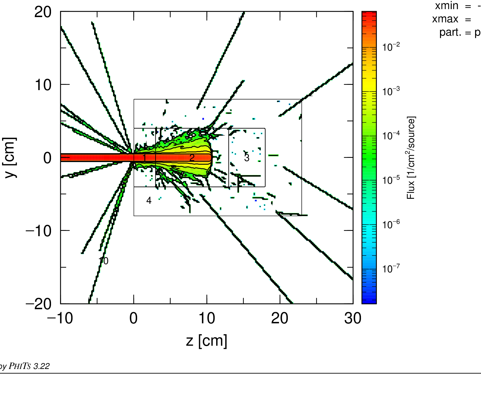
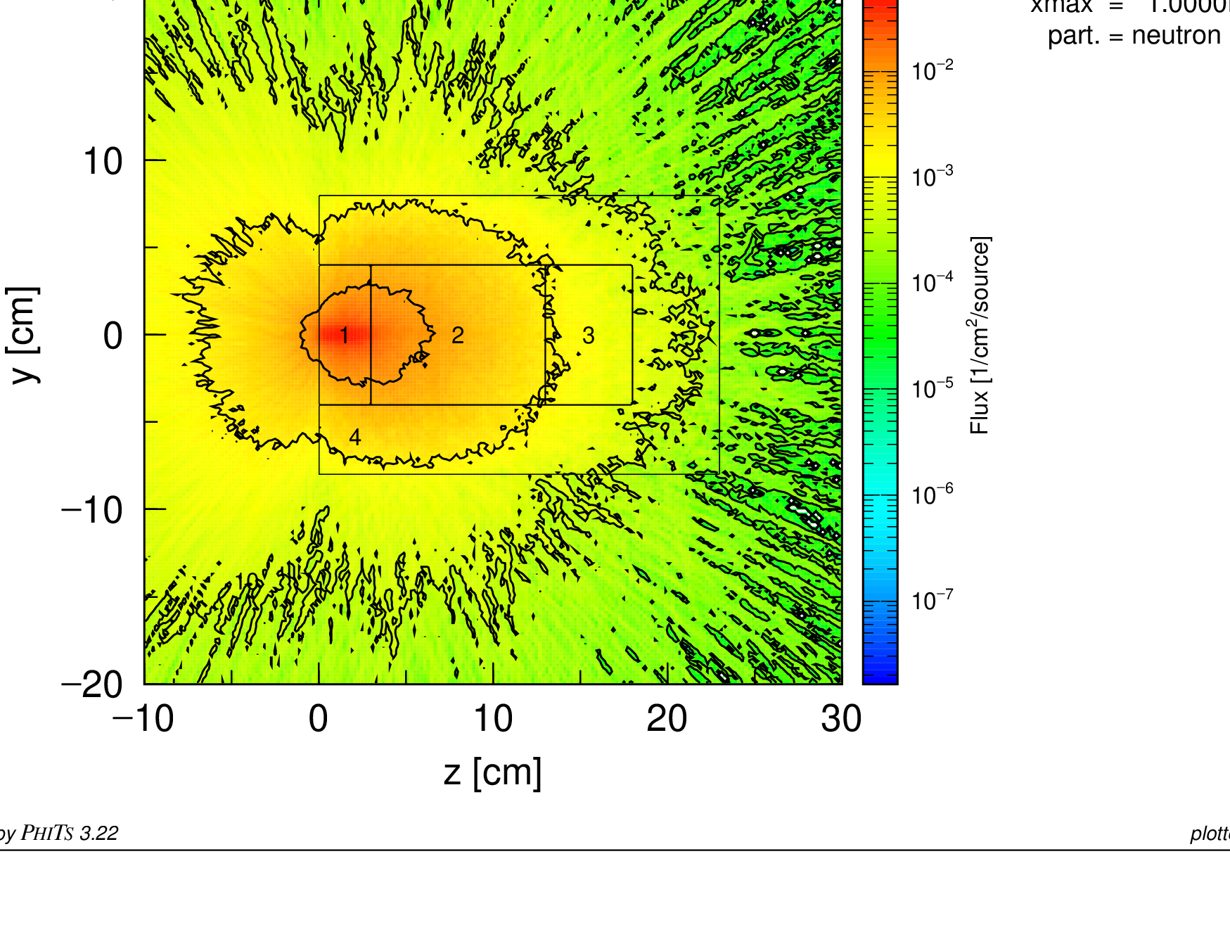
最初の[T-Track]は、ターゲット周辺の粒子フラックスを求める。PHITSを実行すると、図 4.13.3 から 図 4.13.4 の陽子・中性子フラックス分布が得られる。
PHITSは、各[T-Dchain]のfileに指定した名前で3組のDCHAIN入力ファイルを生成する。DCHAINは実行中に一時ファイルを作成するため、同じフォルダー内で複数のDCHAIN計算を同時実行できない。逐次実行するか、別々のフォルダーで実行する必要があり、本例では順番に実行する。DCHAINの設定は、PHITSから引き渡されるものを含め、すべて[T-Dchain]内のパラメータで指定する。
最初の[T-Dchain]では、regメッシュ、出力ファイル名、照射・冷却スケジュール、出力時刻、ビーム強度を指定する。追加設定のiphtout= 2はDCHAIN入力のPHITSOUTに対応し、DCHAINが生成するPHITSの[Source]セクションを出力時刻ごとの別ファイルへ保存する。W_reg_target.inをDCHAINで実行すると通常の出力一式が生成され、*.phtだけは4つの指定出力時刻に対応する4ファイルへ分割される。
2つ目の[T-Dchain]は、regメッシュを3次元のxyzメッシュへ置き換えた点を除き、基本的に同じ設定である。タングステン部は8 cm\(\times\)8 cm\(\times\)3 cmであり、8\(\times\)8\(\times\)3個の1 cm\(^3\)ボクセルへ分割する。
さらに2つのパラメータを追加する。idivs= 4は、DCHAINで各照射期間を分割するサブステップ数を指定する。既定値50は、特に中性子放射化で核種の蓄積を精度よく扱うための保守的な推奨値である。必要な分割数は、重要核種の半減期とtimeevoで指定する照射期間の長さに依存する。本例では放射化の大部分が[T-Yield]の高エネルギー反応生成量に由来するため、多数の分割は不要と判断し、実行時間短縮のため4とする。4.8節 で説明したように、DCHAINの実行時間は領域数(ここでは192)とIDIVSに強く依存する。
もう一つの追加パラメータipltmode= 1は、xyzメッシュを\(xy\)平面で切った放射能分布図をDCHAINに出力させる。W_xyz_target.inをDCHAINで実行する。IDIVSを減らしても領域数が多いため、最初のreg計算より時間を要する。通常の出力に加え、W_xyz_target_pxy.angからW_xyz_target_pxy.epsが生成され、各出力時刻・\(z\)スライスの\(xy\)平面分布が示される。
図 4.13.5 に示すように、放射能はビームが通過する中心部に集中し、冷却時間とともに減少する。また、ビーム軌道周辺の放射化は、ターゲット内の深さが増すほど広がっている。
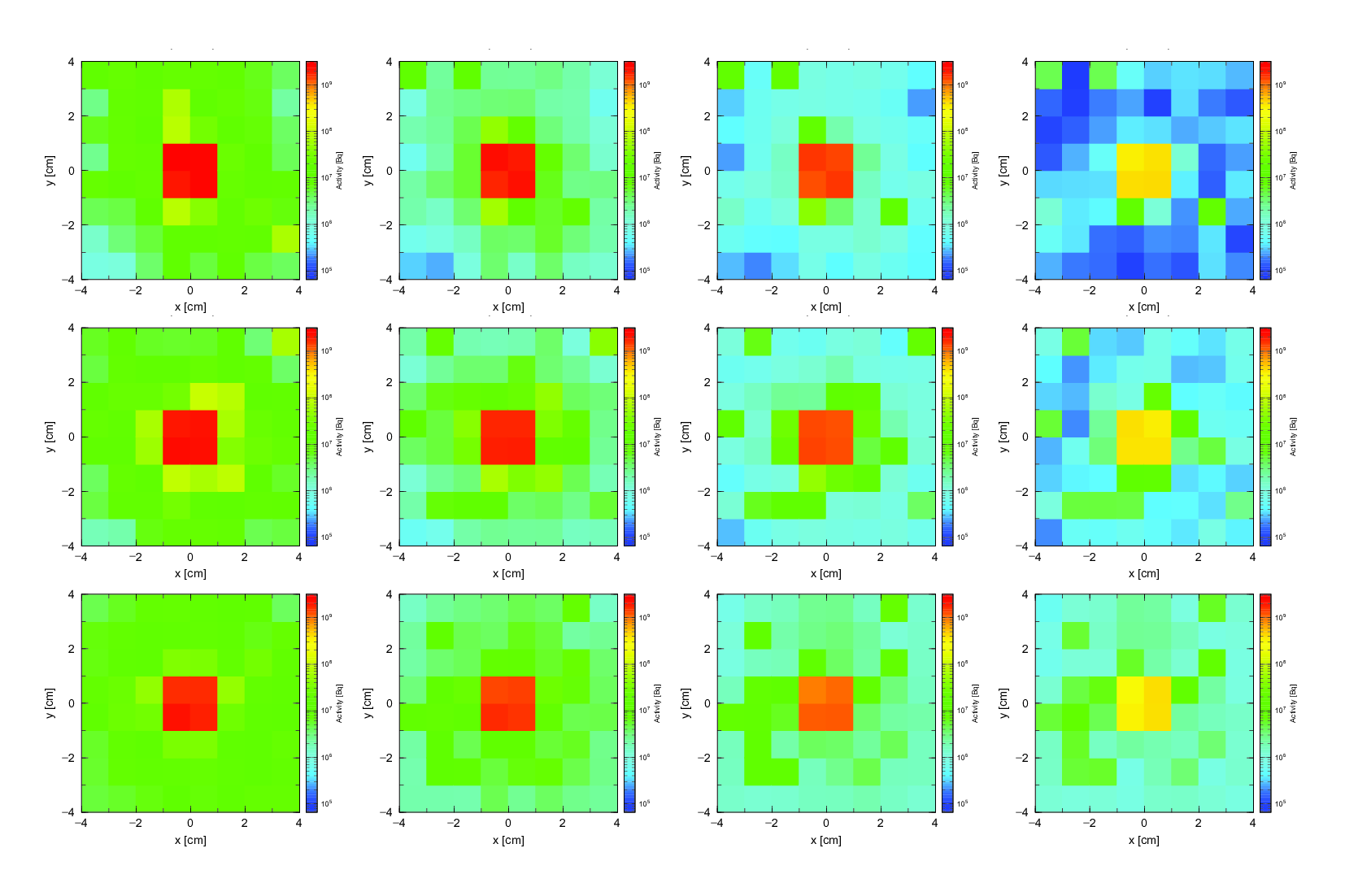
図 4.13.5 タングステンターゲットの放射能分布。縦方向は\(z=0\)–1 cm、1–2 cm、2–3 cmのスライス、横方向は\(t=10\)分(照射終了時)、11分、15分、1時間を示す。
3つ目の[T-Dchain]は2つ目と似ているが、16 cm\(\times\)16 cm\(\times\)23 cmのターゲット全体を覆うxyzメッシュを使用する。1 cm分解能では5,888領域となりDCHAINの実行時間が大幅に増えるため、空間分解能を下げる。このタリーの目的は各材料領域の放射能が時間とともに変化する様子を示すことであるため、\(x\)方向を1ビンにまとめ、\(y\)と\(z\)方向の分解能も粗くする。使用するメッシュは1\(\times\)8\(\times\)12の合計96ボクセルで、各ボクセルの寸法は16 cm\(\times\)2 cm\(\times\)約1.9 cmである。
出力時刻も変更し、照射終了後0秒、10秒、1分、50分とする。idivsは4のまま、ipltmodeを1から4へ変更し、\(x\)方向に切った\(yz\)平面の2次元放射能分布を出力する。whole_target_yz-view.inをDCHAINで実行すると、通常の出力一式が生成される。3つ目の[T-Dchain]ではiphtoutを既定値1から変更していないため、*.phtは1ファイルだけ生成される。whole_target_yz-view_pyz.epsの結果を 図 4.13.6 に示す。ベリリウム領域の放射能は急速に減少する一方、タングステン領域ではより緩やかに減衰する。
ボクセル間の顕著な色のばらつきは、PHITSを10,000ヒストリーしか実行していないことによる大きな統計誤差である。xyzメッシュを細かくするほど、すべてのボクセルで十分な統計精度を得るために必要なヒストリー数も増える。
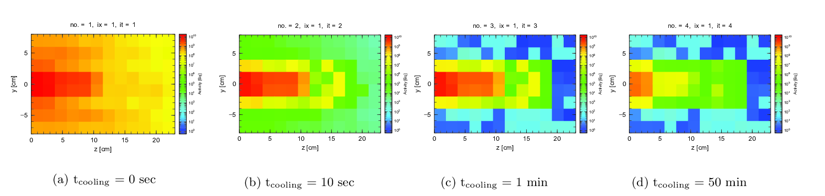
図 4.13.6 照射終了後の各時刻におけるターゲット全体の放射能分布(whole_target_yz-view_pyz.eps)
xyzメッシュでは、1つのボクセルに複数の材料が含まれる場合がある。最初のxyzメッシュはタングステン部だけを覆っていたが、今回は材料境界と一致しないグリッドでターゲット全体を覆っている。DCHAIN入力whole_target_yz-view.inの領域定義冒頭を以下に示す。DCHAINはボクセルを材料ごとに再分割せず、ボクセル内の全材料を均一に混合した1領域として扱う。
! --- calculation region details ---

      imat =      4
   mtscore =      0
   mt-list =      5
   W-180     7.5882E-05
   W-182     1.6756E-02
   W-183     9.0514E-03
   W-184     1.9376E-02
   W-186     1.7975E-02
   mt-list =      3
   H-1       6.6880E-02
   H-2       1.0033E-05
   O-16      3.3446E-02
   mt-list =      4
  Fe-54      4.9642E-03
  Fe-56      7.7928E-02
  Fe-57      1.7997E-03
  Fe-58      2.3951E-04
   mt-list =      1
  Be-9       1.2352E-01
     imesh =      96
   non    ix    iy    iz        fluxs       volume    volmat001    volmat002    volmat003    volmat004
     1     1     1     1   1.2681E+09   6.1333E+01   0.0000E+00   0.0000E+00   0.0000E+00   6.1333E+01
     2     1     2     1   2.8259E+09   6.1333E+01   0.0000E+00   0.0000E+00   0.0000E+00   6.1333E+01
     3     1     3     1   5.6903E+09   6.1333E+01   2.8395E+01   0.0000E+00   0.0000E+00   3.2938E+01
     4     1     4     1   1.7153E+10   6.1333E+01   2.8395E+01   0.0000E+00   0.0000E+00   3.2938E+01
     5     1     5     1   1.7210E+10   6.1333E+01   2.8395E+01   0.0000E+00   0.0000E+00   3.2938E+01
     6     1     6     1   5.6811E+09   6.1333E+01   2.8395E+01   0.0000E+00   0.0000E+00   3.2938E+01
     7     1     7     1   2.7261E+09   6.1333E+01   0.0000E+00   0.0000E+00   0.0000E+00   6.1333E+01
     8     1     8     1   1.2740E+09   6.1333E+01   0.0000E+00   0.0000E+00   0.0000E+00   6.1333E+01
     9     1     1     2   1.5936E+09   6.1333E+01   0.0000E+00   0.0000E+00   0.0000E+00   6.1333E+01
    10     1     2     2   3.7344E+09   6.1333E+01   0.0000E+00   0.0000E+00   0.0000E+00   6.1333E+01
    11     1     3     2   6.9048E+09   6.1333E+01   1.5863E+01   1.3542E+01   0.0000E+00   3.1929E+01
    12     1     4     2   1.5202E+10   6.1333E+01   1.5863E+01   1.3542E+01   0.0000E+00   3.1929E+01
    13     1     5     2   1.4733E+10   6.1333E+01   1.5863E+01   1.3542E+01   0.0000E+00   3.1929E+01
    14     1     6     2   6.8998E+09   6.1333E+01   1.5863E+01   1.3542E+01   0.0000E+00   3.1929E+01
    15     1     7     2   3.7621E+09   6.1333E+01   0.0000E+00   0.0000E+00   0.0000E+00   6.1333E+01
DCHAINが*.phtファイルへ出力したPHITSの[Source]セクションを元のPHITS入力へ挿入し、崩壊放射線の輸送を計算する。ここではregとxyzの両メッシュについて実行し、最終結果を比較する。まずPHITS入力を次のように変更する。崩壊光子は250 MeV陽子より輸送計算が速く、ここでは放射化生成を評価しないため、統計精度を改善する目的でヒストリー数を増やす。
•\(\quad\) バッチ当たりのヒストリー数を1,000から100,000へ増やす。
maxcas   =      100000     # (D=10) number of particles per one batch
maxbch   =          10     # (D=10) number of batches
•\(\quad\) 元の陽子[Source]セクションを無効にする。
[Source] off
   s-type =   1             # mono-energetic axial source
     proj =  proton         # kind of incident particle
       e0 =   250.00        # energy of beam [MeV/u]
•\(\quad\) 室内のセル10、11を真空から空気とコンクリートへ戻す。
$ Room (void)
$ 10  0          -16:(5 -20 15)   $ room + doorway air
$ 11  0          -15:(20 -21 #10) $ outer + maze concrete walls
$ Room (with materials)
10 10 -0.0012  -16:(5 -20 15)   $ room + doorway air
11 11 -2.3     -15:(20 -21 #10) $ outer + maze concrete walls
•\(\quad\) 3つの[T-Dchain]を無効にする。
[T-DCHAIN] off
\(\vdots\)
[T-DCHAIN] off
\(\vdots\)
[T-DCHAIN] off
ターゲット周辺の光子フラックス分布を比較するため、最初の[T-Track]は光子だけを対象とする。まずreg線源を計算することが分かるよう、出力ファイル名の拡張子直前へ_reg-srcを追加する。
file = yz-track_reg-src.out
part = photon
室内の周辺線量当量率分布を計算するため、2つ目の[T-Track]も有効にする。
$ Photon source from DCHAIN output
infl:{W_reg_target_gamma_t3.pht}
$ This needs to come before the "off" source section or it will be skipped.

[Source] off
   s-type =   1             # mono-energetic axial source
     proj =  proton         # kind of incident particle
       e0 =   250.00        # energy of beam [MeV/u]
このタリーは、コンクリート床から高さ2 mまでの範囲で、1 keV~10 MeVの粒子による線量率を求める。factorは出力単位をpSv/sからmSv/hへ変換する。multiplierは、セル10の空気中のフラックスに\(H^*(10)\)フルエンス-線量換算係数を掛け、その他のセルの寄与をゼロにする。angelパラメータは出力図のカラーバー範囲を設定する。
通常、カラーバー範囲は自動設定でもよいが、本例ではregとxyzの結果を同じ尺度で比較するため明示的に固定する。fileも、使用したメッシュを容易に区別できる名前とする。
残る作業は、タングステン部から放出される崩壊光子スペクトルを[Source]として読み込むことである。元の[Source]セクションの前にあるinfl:行を有効にし、W_reg_target_gamma_t3.phtの内容をPHITS入力へ挿入する。
[Title]
Dose from 250MeV protons activating W/H2O/Fe block surrounded in Be

[Parameters]
 icntl    =           0     # (D=0) 3:ECH 5:NOR 6:SRC 7,8:GSH 11:DSH 12:DUMP
 maxcas   =      100000     # (D=10) number of particles per one batch
 maxbch   =          10     # (D=10) number of batches
 file(1)  = c:/phits        # (D=c:/phits) PHITS install folder name
$  required options for DCHAIN
 file(21) = c:/phits/dchain-sp/data # (D=c:/phits/dchain-sp/data) DCHAIN data folder
 jmout    =           1     # (D=0) Density echo, 0:input, 1:number density
 e-mode   =           0     # (D=0) Event generator mode is not recommended for DCHAIN
 igamma   =           3     # (D=2) 0:No, 1:Old, 2:EBITEM, 3:EBITEM+Isomer

$ Photon source from DCHAIN output
infl:{W_reg_target_gamma_t3.pht}
$ This needs to come before the "off" source section or it will be skipped.

[Source] off
   s-type =   1             # mono-energetic axial source
     proj =  proton         # kind of incident particle
       e0 =   250.00        # energy of beam [MeV/u]
       r0 =   0.5000        # radius [cm]
       x0 =   0.0000        # (D=0.0) center position of x-axis [cm]
       y0 =   0.0000        # (D=0.0) center position of y-axis [cm]
       z0 =  -10.000        # minimum position of z-axis [cm]
       z1 =  -10.000        # maximum position of z-axis [cm]
      dir =   1.0000        # z-direction of beam [cosine]

[Material]
$ Tungsten, Density (g/cm3) = 19.300000
M1      74000  1.000000  $  W
$ Water, Density (g/cm3) = 0.998207 ~= 1.0
M2       1000  0.666657  $  H
         8000  0.333343  $  O
$ Iron, Density (g/cm3) = 7.874000
M3      26000  1.000000  $  Fe
$ Beryllium, Density (g/cm3) = 1.848000
M4       4000  1.000000  $  Be
$ Air (dry, sea level), Density (g/cm3) = 0.001205
M10      6000  0.000150  $  C
         7000  0.784431  $  N
         8000  0.210748  $  O
        18000  0.004671  $  Ar
$  Concrete, Ordinary (NIST), Density (g/cm3) = 2.300
M11      1000  0.305330  $  H
         6000  0.002880  $  C
         8000  0.500407  $  O
        11000  0.009212  $  Na
        12000  0.000725  $  Mg
        13000  0.010298  $  Al
        14000  0.151042  $  Si
        19000  0.003578  $  K
        20000  0.014924  $  Ca
        26000  0.001605  $  Fe

set:c1[3]  $ thickness of W portion
set:c2[10] $ thickness of H2O portion
set:c3[5]  $ thickness of Fe portion
set:c4[5]  $ thickness of Be back end
set:c5[4]  $ half side length of inner rectangular prism
set:c6[8]  $ half side length of outer rectangular prism

[Surface]
$ Target components
1 rpp -c5 c5 -c5 c5 0     c1            $ W portion
2 rpp -c5 c5 -c5 c5 c1    c1+c2         $ H2O portion
3 rpp -c5 c5 -c5 c5 c1+c2 c1+c2+c3      $ Fe portion
4 rpp -c5 c5 -c5 c5 0     c1+c2+c3      $ Be inner border
5 rpp -c6 c6 -c6 c6 0     c1+c2+c3+c4   $ Be outer border

$ Room structure
15 rpp -350 -300  -100  200  -100  150  $ inside shield
16 rpp -550 -500  -100  200  -100   50  $ doorway
20 rpp -500  100  -100  200  -100  300  $ inner wall
21 rpp -550  150  -150  250  -150  350  $ outer wall

[Cell]
$ Target
1   1 -19.3    -1               $ W
2   2 -1.0     -2               $ H20
3   3 -7.874   -3               $ Fe
4   4 -1.848    4 -5            $ Be

$ Room (void)
$ 10  0          -16:(5 -20 15)   $ room + doorway air
$ 11  0          -15:(20 -21 #10) $ outer + maze concrete walls
$ Room (with materials)
10 10 -0.0012  -16:(5 -20 15)   $ room + doorway air
11 11 -2.3     -15:(20 -21 #10) $ outer + maze concrete walls

99 -1  21                       $ outer void / particle graveyard

[Volume]   $ required section for DCHAIN
   reg   vol
     1   c1*(2*c5)**2
     2   c2*(2*c5)**2
     3   c3*(2*c5)**2
     4   ((c1+c2+c3+c4)*(2*c6)**2)-((c1+c2+c3)*(2*c5)**2)

[Mat Name Color]
   mat     name     size          color
     0     void     1.00     lightgray
     1    Tungsten  1.00     darkgreen
     2    Water     1.00     pastelcyan
     3    Iron      1.00     orange
     4    Beryllium 1.00     pastelviolet
    10    Air       1.00     {-0.9}
    11    Concrete  1.00     gray

$ Beam settings to be used in [T-Dchain] tallies
set:c11[100.0]                           $ beam current (nA)
set:c12[ c11 * 1.0e-9 / (1.602177e-19) ] $ beam power (source/sec)

[T-DCHAIN] off
  title = W target (reg)
  mesh = reg
  reg = 1
  file = W_reg_target.in     # file name of dchain input file
  timeevo =    2             # time evolution / irradiation schedule
    10.0 m 1.0
    50.0 m 0.0
  outtime =    4             # output times
    10.0 m
    -1 m
    -5 m
    -50 m
  amp = c12                  # (D=1.0) Source Intensity(source/sec)
  iphtout = 2                # (D=1) 2 = separate [Source] output to files for each time

[T-DCHAIN] off
  title = W target (xyz)
  mesh = xyz
  x-type = 2
      nx = 8
    xmin = -c5
    xmax =  c5
  y-type = 2
      ny = 8
    ymin = -c5
    ymax =  c5
  z-type = 2
      nz = 3
    zmin = 0
    zmax = c1
  file = W_xyz_target.in     # file name of dchain input file
  timeevo =    2             # time evolution / irradiation schedule
    10.0 m 1.0
    50.0 m 0.0
  outtime =    4             # output times
    10.0 m
    -1 m
    -5 m
    -50 m
  amp = c12                  # (D=1.0) Source Intensity(source/sec)
  idivs = 4                  # (D=50) number of calculation substebs used in irradiation
  iphtout = 2                # (D=1) 2 = separate [Source] output to files for each time
  ipltmode = 1               # (D=0) enable DCHAIN 2D xy activity plot

[T-DCHAIN] off
  title = Whole target structure
  mesh = xyz
  x-type = 2
      nx = 1
    xmin = -c6
    xmax =  c6
  y-type = 2
      ny = 8
    ymin = -c6
    ymax =  c6
  z-type = 2
      nz = 12
    zmin = 0
    zmax = c1+c2+c3+c4
  file = whole_target_yz-view.in  # file name of dchain input file
  timeevo =    2             # time evolution / irradiation schedule
    10.0 m 1.0
    50.0 m 0.0
  outtime =    4             # output times
    10.0 m
    -10 s
     -1 m
    -50 m
  amp = c12                  # (D=1.0) Source Intensity(source/sec)
  idivs = 4                  # (D=50) number of calculation substebs used in irradiation
  ipltmode = 4               # enable DCHAIN 2D yz activity plot

[T-Track]
  title = proton, neutron, and photon distributions
    mesh = xyz
  x-type = 2
    xmin = -10
    xmax =  10
      nx = 1
  z-type = 2
    zmin = -10
    zmax =  30
      nz = 200
  y-type = 2
    ymin = -20
    ymax =  20
      ny = 200
  e-type = 2
    emin = 0
    emax =  2000
      ne = 1
    axis = yz
    file = yz-track_reg-src.out
    part = photon
    unit = 1
  2D-type =  7   # 1:Cont, 2:Clust, 3:Color, 4:xyz, 5:mat, 6:Clust+Cont, 7:Col+Cont
  gshow =    3   # 0: no 1:bnd, 2:bnd+mat, 3:bnd+reg 4:bnd+lat
  epsout = 1     # automatically generate eps plot

[T-Track]
  title = Ambient dose equivalent H*(10) [mSv/hr] room map
  mesh = xyz
  x-type = 2
      nx =  140
    xmin = -550
    xmax =  150
  y-type = 2
      ny = 1
    ymin = -100
    ymax =  100
  z-type = 2
      nz =  100
    zmin = -150
    zmax =  350
    unit = 1
    axis = xz
  e-type = 3
      ne = 1
    emin = 0.001
    emax = 10
  file = room-dose_reg-src.out
  set:c20[3600/1.0E+09]
  factor = c20       $ convert pSv/sec to mSv/hr
  multiplier = 6     $ number of regions using multiplier
     mat    mset1
     1    ( 0 -200 ) $ Zero out regions where we don't
     2    ( 0 -200 ) $   care about the dose (inside walls
     3    ( 0 -200 ) $   and the target).
     4    ( 0 -200 )
     10   ( 1 -200 ) $ We only want to tally dose rate in air.
     11   ( 0 -200 )
  2D-type =  7   # 1:Cont, 2:Clust, 3:Color, 4:xyz, 5:mat, 6:Clust+Cont, 7:Col+Cont
  gshow =    1   # 0: no 1:bnd, 2:bnd+mat, 3:bnd+reg 4:bnd+lat
  epsout = 1         $ automatically generate eps plot
  $ Set bounds of ANGEL plot color bar and make axis labels bigger
  angel = cmin(1.0E-5) cmax(1.0E+1)
  sangel = 2
  x: {\Large z [cm]}
  y: {\Large x [cm]}

[T-Gshow]
  mesh = xyz
  x-type = 2
      nx = 280
    xmin = -550
    xmax =  150
  y-type = 2
      ny = 1
    ymin =  -5
    ymax =  5
  z-type = 2
      nz = 200
    zmin = -150
    zmax =  350
  axis = zx
  file = room_geometry_cross-section.ang
  output = 2
  epsout = 1

[T-Gshow]
  mesh = xyz
  x-type = 2
    xmin = -20
    xmax =  20
      nx = 200
  z-type = 2
    zmin = -10
    zmax =  30
      nz = 200
  y-type = 2
    ymin = -10
    ymax =  10
      ny = 1
  axis = zx
  file = target_geometry.ang
  output = 2
  epsout = 1

[End]
[T-Dchain]でiphtout= 2(DCHAINではPHITSOUT= 2)を選択したため、全領域の崩壊放射線スペクトルは出力時刻ごとの別ファイルへ保存されている。ファイル名のt3は3番目の出力時刻、すなわち照射終了5分後を表す。iphtoutを既定値1のままにした場合は、単一の*.phtファイル内で3番目の[Source]セクションに対応する行範囲をinfl:に指定する必要がある。
ただし、PHITSを実行する前にW_reg_target_gamma_t3.phtの[Source]セクションを一部修正する必要がある。冒頭部分を以下に示す。
この[Source]はs-type = 5(s-type = 2と同等)を使用する。この形式では対象セルを選び、そのセルを囲む直方体を指定する。PHITSは各ヒストリーについて直方体内の点をランダムに選び、指定セル内の点が得られるまで試行する。reg =のセル番号はDCHAINが自動設定するが、regメッシュからセルの空間境界は分からないため、DCHAINは直方体を自動生成できない。
c <>-<>-<>-<>-<>-<>-<>-<>-<>-<>-<>-<>-<>-<>-<>-<>-<>-<>-<>
c <>-<>   no.     1  regionwise calculation data     <>-<>
c <>-<>   region label : DUMMY001                    <>-<>
c <>-<>-<>-<>-<>-<>-<>-<>-<>-<>-<>-<>-<>-<>-<>-<>-<>-<>-<>
c      no.  3   region=       1   output time=        15 [m]  (after the last shutdown=         5 [m])
c      --------------------------------------------------------------------------------
[ S o u r c e ]
 totfact =   2.9969E+10  $ total number of gamma-rays (n/sec/cc) x volume (cc)
  s-type =   5
    proj = photon
     reg =        1 $ This cell ID  should be revised for lattice  or combined cell case
      x0 =        $ Input minimum x of the region here
      x1 =        $ Input maximum x of the region here
      y0 =        $ Input minimum y of the region here
      y1 =        $ Input maximum y of the region here
      z0 =        $ Input minimum z of the region here
      z1 =        $ Input maximum z of the region here
     dir = all
  e-type = 4
      ne =     28
$     Energy  Flux (arbitrary unit)
$             ^^^^ Energy spectra (n/sec/cc) based on activity concentration (Bq/cc)
      0.0010  1.4968E+06
      0.0100  2.2244E+05
      0.0200  3.3342E+06
      0.0300  3.7151E+06
      0.0450  1.3536E+06
      0.0600  1.2430E+06
      0.0700  2.6622E+05
      0.0750  5.2830E+06
      0.1000  1.1886E+07
      0.1500  1.0705E+07
      0.2000  1.6758E+07
      0.3000  8.4243E+06
      0.4000  5.8011E+06
      0.4500  5.3487E+06
      0.5100  4.4978E+07
      0.5120  4.0259E+06
      0.6000  3.0961E+06
      0.7000  2.0139E+06
      0.8000  9.2412E+06
      1.0000  7.7230E+06
      1.3300  3.3297E+05
      1.3400  3.7883E+06
      1.5000  1.2398E+06
      1.6600  2.2654E+06
      2.0000  5.7494E+05
      2.5000  1.7159E+05
      3.0000  7.6359E+05
      3.5000  3.3674E+04
      4.0000
したがって、[Source]セクションへ直方体の境界を手動で追加する。線源点の棄却を減らすには、対象セル全体を含む範囲で直方体をできるだけ小さくする。本例の対象セル自体が直方体であるため、次のように正確な寸法を指定できる。
reg =        1 $ This cell ID  should be revised for lattice  or combined cell case
 x0 =  -4    $ Input minimum x of the region here
 x1 =   4    $ Input maximum x of the region here
 y0 =  -4    $ Input minimum y of the region here
 y1 =   4    $ Input maximum y of the region here
 z0 =   0    $ Input minimum z of the region here
 z1 =   3    $ Input maximum z of the region here
totfactは、PHITSのタリー結果を実際の崩壊光子放出率へ規格化する。本例のタングステン領域全体の放出率は2.9969E+10 photons/sである。これは、*.actファイルに記載された体積光子放出率1.5609E+08\(\gamma\)/(cm\(^3\cdot\)s)に、領域体積8 cm\(\times\)8 cm\(\times\)3 cm = 192 cm\(^3\)を掛けた値である。
1.5609E+08\(\gamma\)/(cm\(^3\cdot\)s)\(\times\)192 cm\(^3\)= 2.9969E+10\(\gamma\)/s
total gamma-ray flux 1.5609E+08 +/- 7.5486E+06 ( 4.84%) [n/s/cc]
[T-Track]出力の単位換算を説明する。unit = 1の基本単位は、線源粒子当たりの\(\#\)/cm\(^2\)である。[Source]のtotfactによって\(\gamma\)/s単位の放出率で規格化する。さらに、[T-Track]のmultiplierで使用するフルエンス-線量換算係数の単位はpSv\(\cdot\)cm\(^2\)/particle(ここではparticle = \(\gamma\))である。最後にfactorで、時間を秒から時間へ、線量をpSvからmSvへ換算する。したがって、最終出力単位は次式のようにmSv/hとなる。
[Source]の準備が完了したら、PHITS入力dchain_ex-dose.inpを実行する。2つの[T-Track]から 図 4.13.7 から 図 4.13.8 までの結果が得られる。カラーバーには既定の「Flux [1/cm\(^2\)/source]」と表示されるが、実際の単位は上記の規格化と換算を反映する。図 4.13.7 の光子フラックスは\(\gamma\)/(cm\(^2\cdot\)s)、図 4.13.8 の周辺線量当量率はmSv/hである。ラベルや図の大きさは*.outを編集し、ANGELを再実行して変更できる。カラーバーのラベル指定はファイル末尾付近にある。
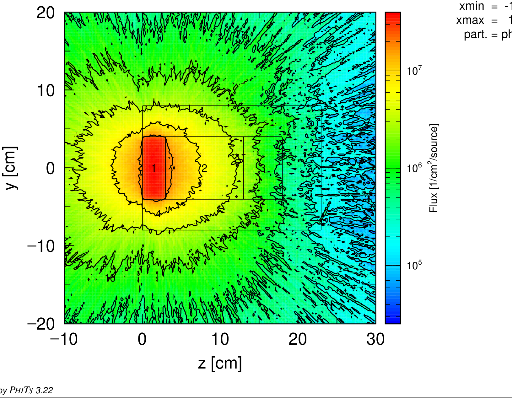
図 4.13.7 ターゲット周辺における放射化タングステン由来の崩壊光子フラックス [\(\frac{\gamma}{\text{cm}^2\cdot\text{s}}\)]
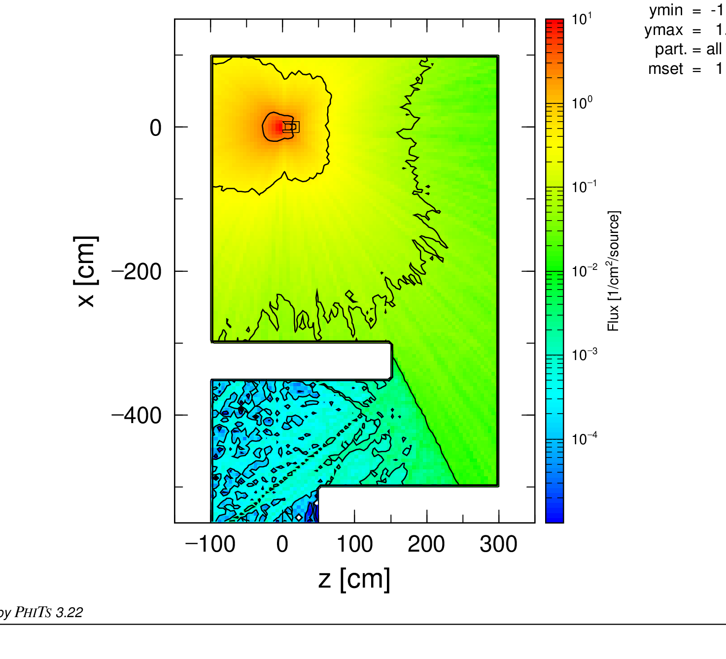
図 4.13.8 室内の\(\dot{H}^*(10)\)分布 [mSv/h]
比較のため、mesh = xyzの線源について同じPHITS計算を行う。入力の変更点は次の2点だけである。
•\(\quad\) infl:で読み込むファイルを、同じ出力時刻のxyzメッシュ計算で生成した*.phtへ変更する。
$ Photon source from DCHAIN output
infl:{W_xyz_target_gamma_t3.pht}
$ This needs to come before the "off" source section or it will be skipped.
•\(\quad\) 2つの[T-Track]の出力ファイル名を、xyz線源を使用したことが分かる名前へ変更する。
file = yz-track_xyz-src.out
file = room-dose_xyz-src.out
変更はこれだけである。regメッシュと異なり、xyzメッシュのグリッド境界はPHITSのタリー出力からDCHAINへ渡される。そのため、DCHAINが生成する*.phtには各線源ボクセルの直方体境界がすでに記載されており、手動入力は不要である。xyz用*.phtの構造を理解するため、W_xyz_target_gamma_t3.phtの最初の線源部分を以下に示す。
c <>-<>-<>-<>-<>-<>-<>-<>-<>-<>-<>-<>-<>-<>-<>-<>-<>-<>-<>
c <>-<>   no.     1  regionwise calculation data     <>-<>
c <>-<>   region label : xyz.000001                  <>-<>
c <>-<>-<>-<>-<>-<>-<>-<>-<>-<>-<>-<>-<>-<>-<>-<>-<>-<>-<>
c      no.  3   region=       1   output time=        15 [m]  (after the last shutdown=         5 [m])
c      ---------------------------------------------------------------------------------
 [ S o u r c e ]
<Source> =   2.8071E+05  $ total number of gamma-rays (n/sec/cc) x volume (cc) in this xyz voxel at this time
 totfact =   2.8071E+05  $ total number of gamma-rays (n/sec/cc) x volume (cc) summed over all preceeding regions at this time; only totfact from final <source> will be used
  s-type =   5
    proj = photon
     reg = all  $ This cell ID should be revised for lattice or combined cell case
      x0 = -4.000000E+00 $ Minimum x of the region
      x1 = -3.000000E+00 $ Maximum x of the region
      y0 = -4.000000E+00 $ Minimum y of the region
      y1 = -3.000000E+00 $ Maximum y of the region
      z0 =  0.000000E+00 $ Minimum z of the region
      z1 =  1.000000E+00 $ Maximum z of the region
     dir = all
  e-type = 4
      ne =     25
$     Energy  Flux (arbitrary unit)
$             ^^^^ Energy spectra (n/sec/cc) based on activity concentration (Bq/cc)
      0.0010  1.2268E+01
      0.0100  2.6172E+01
      0.0200  3.0745E+01
      0.0300  3.5958E+01
      0.0450  5.2974E-03
      0.0600  5.1652E+02
      0.0700  3.4553E+04
まず、特定のセル番号ではなくreg = allを使用する。xyzメッシュの1ボクセルに複数セルの一部が含まれる可能性があるためである。さらに、<Source> = 2.8071E+05が追加され、ファイルにはxyzグリッドの全ボクセルに対応する<Source>が並ぶ。このためreg用ファイルより大幅に長くなる。これは複数の線源を同時に使用するPHITSのマルチソース構文である。
各<Source>の値は、他の線源に対する相対強度を表し、PHITSで読み込む際に合計1へ規格化される。タリー結果を実際の放出率へ規格化するのはtotfactである。各<Source>にtotfactが記載されているが、PHITSが[Source]セクション全体へ適用するのは最後に記載された値だけである。途中のtotfactは、そのボクセルまでの放出率を累積した値である。最後のボクセルの冒頭を以下に示す。
c <>-<>   no.   192  regionwise calculation data     <>-<>
c <>-<>   region label : xyz.000192                  <>-<>
c <>-<>-<>-<>-<>-<>-<>-<>-<>-<>-<>-<>-<>-<>-<>-<>-<>-<>-<>
c      no.  3   region=     192   output time=        15 [m]  (after the last shutdown=         5 [m])
c      ---------------------------------------------------------------------------------
<Source> =   1.3708E+06  $ total number of gamma-rays (n/sec/cc) x volume (cc) in this xyz voxel at this time
 totfact =   2.9969E+10  $ total number of gamma-rays (n/sec/cc) x volume (cc) summed over all preceeding regions at this time; only totfact from final <source> will be used
  s-type =   5
    proj = photon
     reg = all  $ This cell ID should be revised for lattice or combined cell case
      x0 =  3.000000E+00 $ Minimum x of the region
      x1 =  4.000000E+00 $ Maximum x of the region
      y0 =  3.000000E+00 $ Minimum y of the region
      y1 =  4.000000E+00 $ Maximum y of the region
      z0 =  2.000000E+00 $ Minimum z of the region
      z1 =  3.000000E+00 $ Maximum z of the region
     dir = all
最後のボクセルのtotfact= 2.9969E+10は、regメッシュの[Source]に記載された全光子放出率と一致する。これは同じタングステン領域の総放出率を、空間分割の異なる2つの方法で表しているためである。この最後の値が全タリー結果の規格化に使用される。更新したdchain_ex-dose.inpをPHITSで実行すると、実際に採用されたtotfactをphits.outの入力エコーで確認できる。
[ Source ]
  totfact =  2.99690E+10    # (D=1.0) global factor
マルチソースでは、totfactの符号によって各<Source>のサンプリング方法が変わる。正の場合は、すべての線源粒子を同じウェイトで生成し、各<Source>を相対強度に比例した頻度で選ぶ。強度の大きい線源ほど頻繁に選ばれる。負の場合は、すべての<Source>を同じ頻度で選び、生成粒子のウェイトを各線源の相対強度に応じて調整する。既定では正である。xyzメッシュ内の放射能が数桁にわたって変化し、低放射能のボクセルも十分にサンプリングしたい場合は、最後のtotfactだけを負へ変更できる。
なお、xyzメッシュで[T-Dchain]のouttime(DCHAINではITOUT)を複数指定する場合、iphtout= 2(PHITSOUT= 2)は実質的に必須である。DCHAINは領域ごとに計算し、1領域の全時刻を出力してから次の領域へ進む。既定の*.actと、分割しない*.phtもこの順序で構成される。一方、この輸送計算に必要なのは、1つの時刻における全領域の崩壊スペクトルである。iphtout= 1では、対象時刻に対応する192個の<Source>について、個別の行範囲をinfl:へ指定しなければならない。別の方法は、outtimeを必要な1時刻だけに限定することである。
xyzマルチソースでPHITSを実行した結果を 図 4.13.9 から 図 4.13.10 に示す。
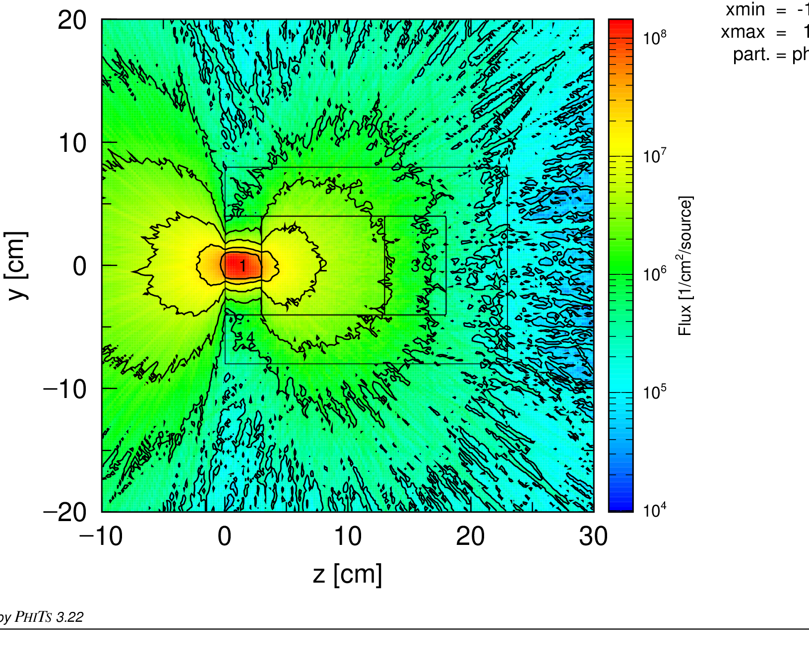
図 4.13.9 ターゲット周辺における放射化タングステン由来の崩壊光子フラックス [\(\frac{\gamma}{\text{cm}^2\cdot\text{s}}\)]
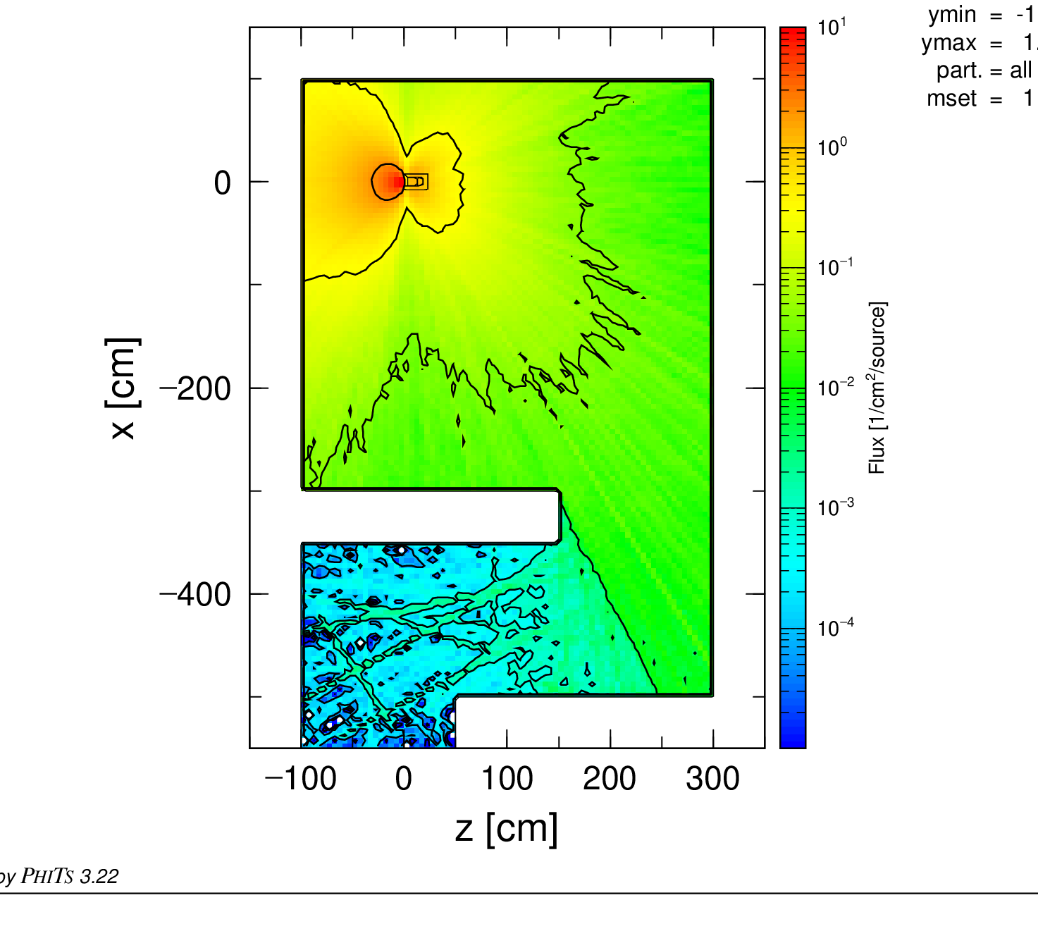
図 4.13.10 室内の\(\dot{H}^*(10)\)分布 [mSv/h]
regメッシュでは、放射能と崩壊光子放出をタングステン領域全体へ一様に分布させる。xyzメッシュでは、DCHAINの2次元放射能分布ですでに確認したように、放出位置がビーム軌道付近へ集中する。多くの光子がタングステン中心部で発生し、ターゲット外へ出る前に減衰するため、自己遮蔽効果が大きくなる。その結果、室内へ到達する光子が減り、周辺線量当量率もregの結果より低くなる。
両計算で一次陽子と崩壊光子のヒストリー数は同じであるが、xyzの結果はregより統計的なばらつきが大きく見える。xyzでは同数の線源光子のうち、中心部で発生して室内へ到達する前に吸収される割合が高いためである。
統計精度はPHITSのヒストリー数を増やすことで改善できる。図 4.13.11 から 図 4.13.14 に、regとxyzの両方でヒストリー数を100万から5,000万へ増やした結果を示す。カラーバーのラベルもANGELで修正している。ターゲット周辺の光子フラックスに対する自己遮蔽と、それに伴う室内\(\dot{H}^*(10)\)の低下がより明確に分かる。
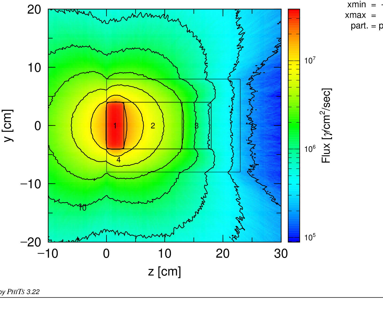
図 4.13.11 reg:ターゲット周辺の崩壊光子フラックス [\(\frac{\gamma}{\text{cm}^2\cdot\text{s}}\)]
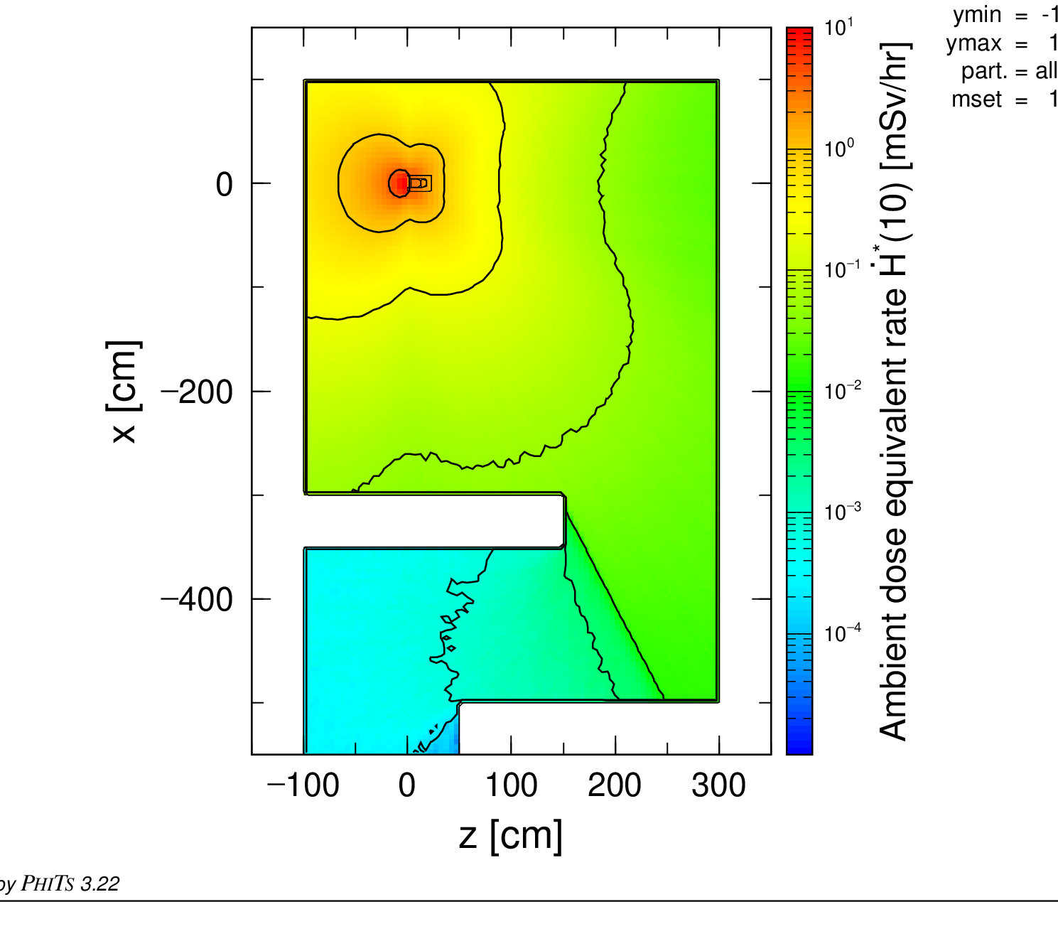
図 4.13.12 reg:室内の\(\dot{H}^*(10)\)分布 [mSv/h]
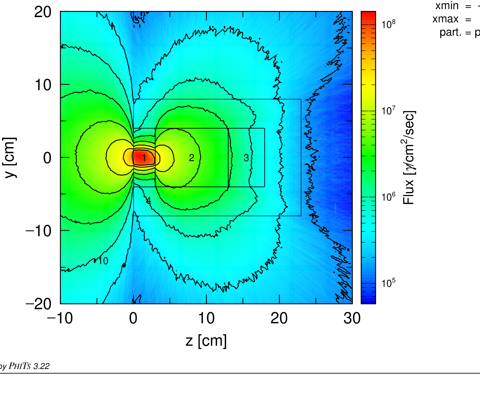
図 4.13.13 xyz:ターゲット周辺の崩壊光子フラックス [\(\frac{\gamma}{\text{cm}^2\cdot\text{s}}\)]
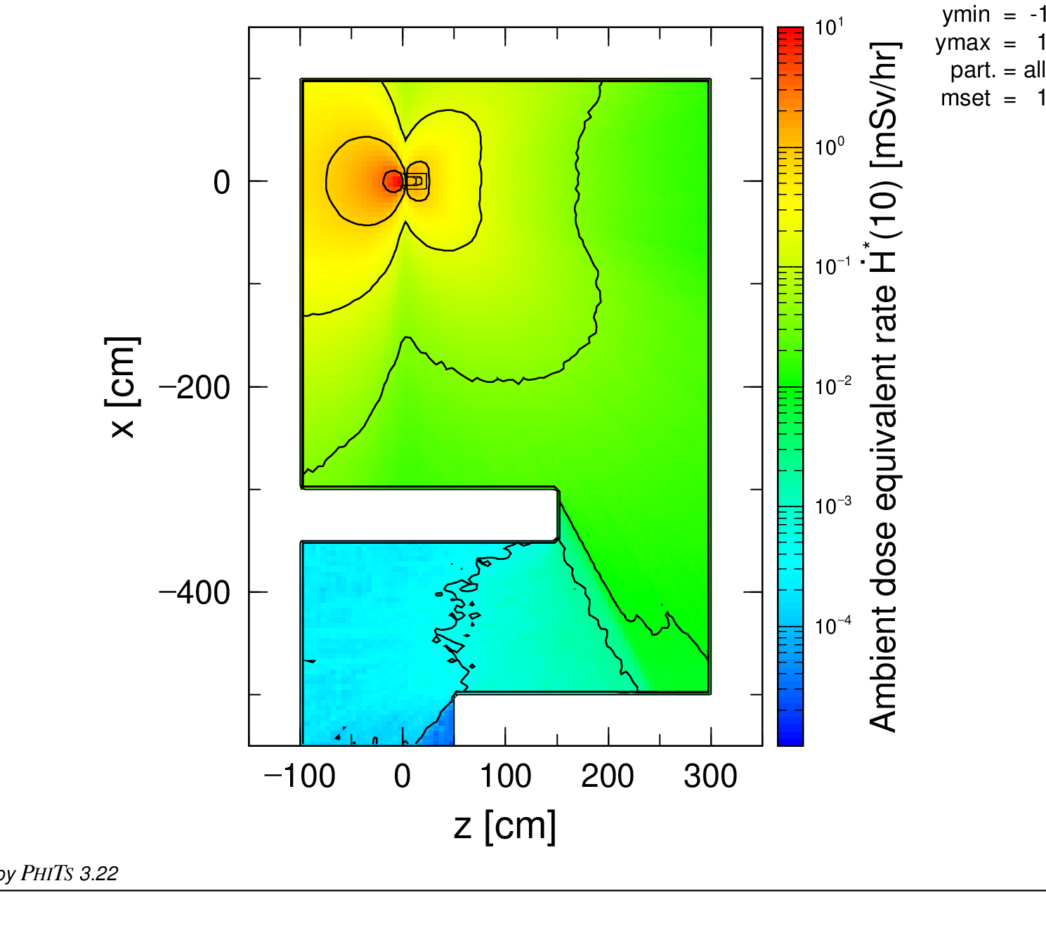
図 4.13.14 xyz:室内の\(\dot{H}^*(10)\)分布 [mSv/h]
説明のため、図 4.13.15 から 図 4.13.16 に、5000万ヒストリーのxyzメッシュ計算でtotfactを負にした場合の結果を示す。ここでは、W_xyz_target_gamma_t3.phtの最後のtotfactの符号だけを変更した。直感に反して、ターゲット端部に近いボクセルがより多くサンプリングされても、統計精度は悪化している。*.gsoと*.actファイルを調べると、線量率への寄与と透過力が大きい光子は、主としてタングステン中の高エネルギービーム反応で生成した核種から放出され、xyzメッシュではターゲット中心付近のボクセルに集中していることが分かる。負のtotfactでは全ボクセルを同じ頻度で選ぶため、放射能が最も高い中心ボクセルのサンプリング頻度も低下する。前述の 放射能分布 に示す \(8\times8\) グリッドでは、中心4ボクセルがビーム反応による放射化の大部分を占めるが、負のtotfactではヒストリーの6.25 %でしか選択されず、正の場合よりサンプリング頻度が低くなる。
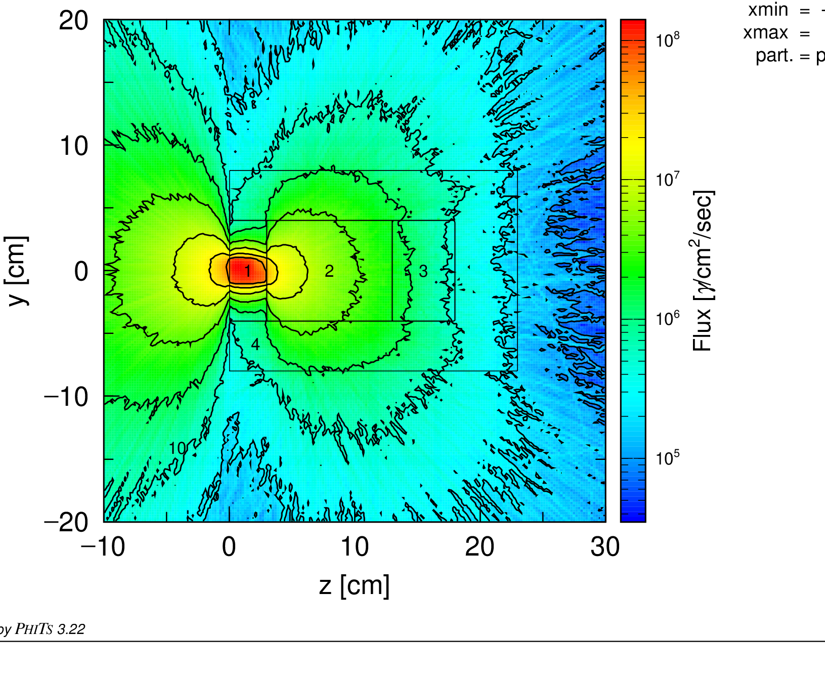
図 4.13.15 xyz (totfact < 0):ターゲット周辺の崩壊光子フラックス [\(\frac{\gamma}{\text{cm}^2\cdot\text{s}}\)]
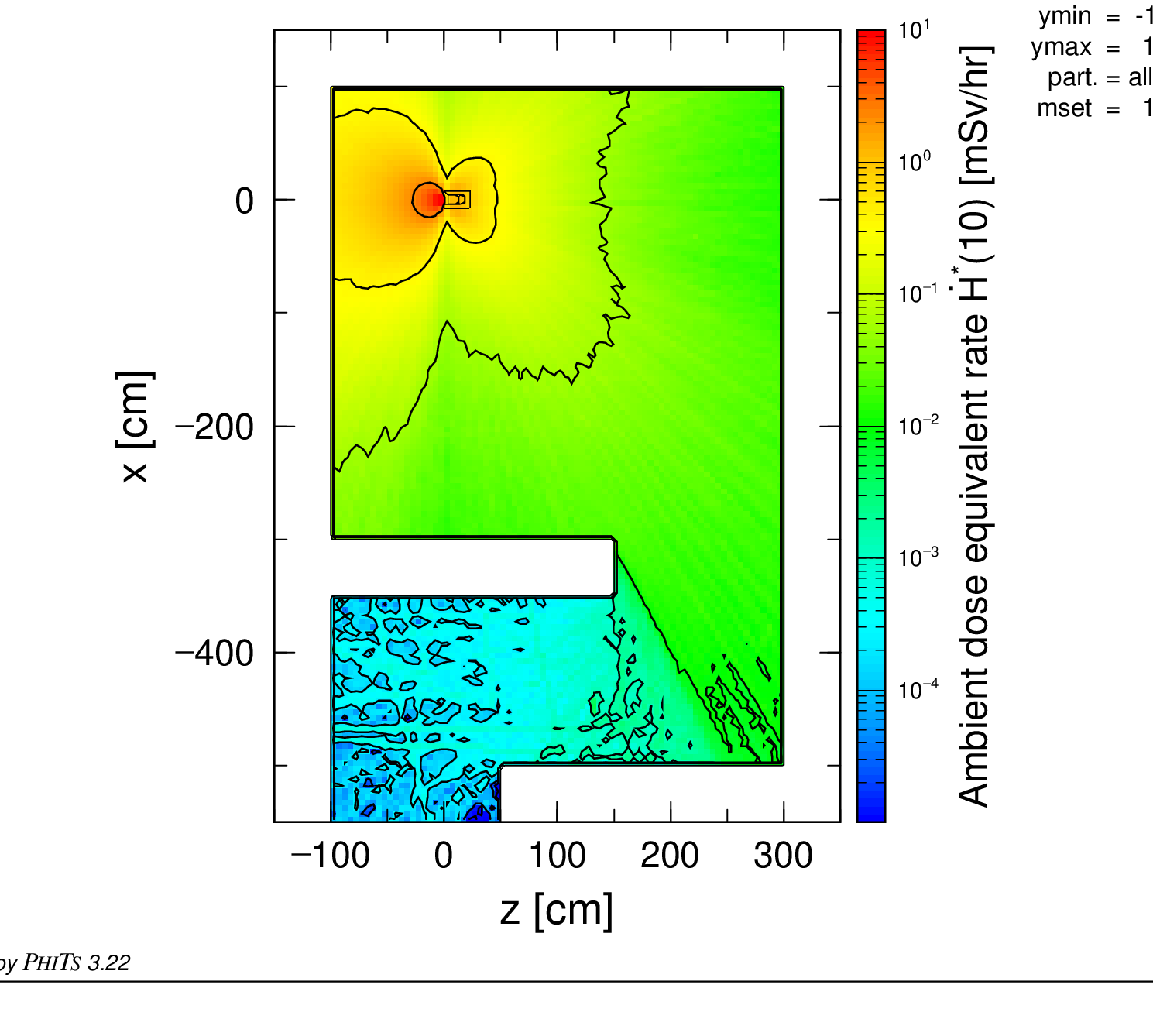
図 4.13.16 xyz (totfact < 0):室内の\(\dot{H}^*(10)\)分布 [mSv/h]
どちらの符号が適切かは、計算体系、メッシュ分解能、放射化分布、放射化に寄与する反応、対象とする崩壊放射線、二段階目のPHITS計算で評価する量に依存する。例えば、中心部の放射化が強くても、物体が厚く高密度で中心からの放射線がほとんど外へ出ない場合には、totfactを負にして、放射能は低いものの表面に近い多数のボクセルをより頻繁にサンプリングする方が、周辺線量評価の統計を改善できる可能性がある。一般には、対象タリーへ寄与する粒子数が最大になるようにtotfactの符号を選ぶ必要があるが、どちらが効率的かは必ずしも事前には明らかでない。