7.2. [ T-Cross ] section
This tally can be used to obtain the current or flux, actually the fluence, on any specified surface. In this tally, a particle crossing the surface simply adds 1 to the current and \(1/\cos\theta\) to the flux, where \(\theta\) is the angle between the direction of the particle trajectory and the normal vector to the surface. In PHITS, the current and flux are similar but distinct physical quantities; they differ in terms of the surface element used to calculate the number of the particles crossing per unit area. The current is evaluated by dividing by the area of the surface \(S\) shown in Fig. 7.2.1; by contrast, the flux is calculated by dividing by \(S\cos\theta\). The value of \(S\) is given in the mesh type subsection as area for mesh=reg and is calculated automatically for the r-z and xyz meshes.
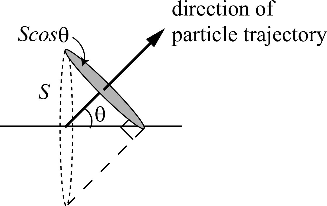
Fig. 7.2.1 Relation between the areas \(S\) and \(S\cos\theta\).
As the flux in this tally is evaluated by weighting by \(1/\cos\theta\), the result is equivalent to that obtained from the [t-track] tally for an extremely thin region. Consequently, information on the detector response in the specified surface can be obtained from the [t-cross] tally. Multiplying the flux by a cross section, in units of cm^2, of the detector enables estimation of the number of counts in the response.
value |
explanation |
reg, r-z, xyz |
Mesh type. A mesh type subsection is required below this option. |
If a boundary of geometry coincides with a tally plane at a cylindrical surface in r-z mesh or at a rotated surface in xyz mesh, the tally results might be underestimated due to the problem of significant digits. In such cases, the mesh size should be changed slightly so that it does not coincide with the boundary plane.
value |
explanation |
all (default), particle name |
Tally particle. |
value |
explanation |
1, 2, 3, 4, 5 |
Energy mesh. See Section 6.6.1 for mesh subsection format. |
value |
explanation |
MeV (default), keV, eV, nm, A0, keV/um |
Unit of energy mesh. nm specifies wavelength in nanometers, A0 specifies wavelength in angstroms. For massive particles, the de Broglie wavelength is used. When using nm or A0, unit must be 1, 4, 11, or 14. keV/um converts the energy axis to LET (equivalent to eng2let=1). |
value |
explanation |
(optional) |
0 (default): Do not convert energy defined by e-type to LET. 1: Convert energy to LET (keV/um). Set eng2let=1 and axis=let when you want to output the results as a function of LET. |
value |
explanation |
1, 2, 3, 4, 5 (optional) |
Time mesh. See Section 6.6.1 for mesh subsection format. |
value |
explanation |
1, 2, -1, -2 (optional) |
Angle mesh, =1,2 for cosine mesh and =-1,-2 for angle mesh in units of degree. See Section 6.6.1 for mesh subsection format. Required for output=a-curr or output=oa-curr. |
The current for a specified angle can be obtained using the angle mesh shown in Fig. 7.2.2. In cases where unit=4,5,6,14,15,16, the output is given as a quantity per solid angle, in steradians, calculated using the mesh size of the angle bin defined in the angle mesh subsection.
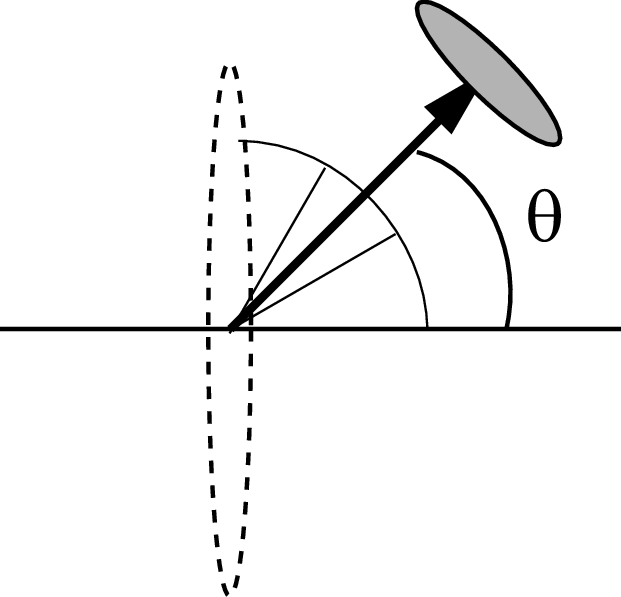
Fig. 7.2.2 Schematic of tally using angle mesh.
value |
explanation |
0 (default), 1, 2, 3 |
Select the angle in a-type mesh. 0: The angle between the normal vector to the surface and the direction of the particle trajectory, \(\theta\). 1: The angle between the x-axis and the direction of the particle trajectory. 2: The angle between the y-axis and the direction of the particle trajectory. 3: The angle between the z-axis and the direction of the particle trajectory. |
value |
explanation |
1, 2, 3, 4, 5, 6 |
1: [1/cm^2/source] 2: [1/cm^2/MeV/source] 3: [1/cm^2/Lethargy/source] 4: [1/cm^2/sr/source] 5: [1/cm^2/MeV/sr/source] 6: [1/cm^2/Lethargy/sr/source] |
11, 12, 13, 14, 15, 16 |
11: [1/cm^2/nsec/source] 12: [1/cm^2/MeV/nsec/source] 13: [1/cm^2/Lethargy/nsec/source] 14: [1/cm^2/sr/nsec/source] 15: [1/cm^2/MeV/sr/nsec/source] 16: [1/cm^2/Lethargy/sr/nsec/source] |
Lethargy in unit=3,6,13,16 is the natural logarithmic unit of energy defined by \(\ln(E_{\rm ref}/E)\) using a reference energy \(E_{\rm ref}\) and the particle energy \(E\). Setting these units enables obtaining results in units of Lethargy, which are given as Lethargy widths, \(\ln(E_{\rm high}/E_{\rm low})\), for each energy bin in the energy mesh subsection. Here \(E_{\rm high}\) and \(E_{\rm low}\) are the maximum and minimum values of the energy bins, respectively.
In unit=4,5,6,14,15,16, sr denotes steradians as the solid angle unit.
value |
explanation |
eng, let, reg, x, y, z, r |
x axis value of output data. |
cos, the, t |
Angle, cosine or \(\theta\) in degree, and time mesh. |
xy |
2-dimensional. |
yz, xz, rz |
2-dimensional, only for enclos=1. |
value |
explanation |
(optional, |
The type of data to be displayed on the same page of the image output file. Parameters that can be defined in axis can be specified. |
value |
explanation |
|
Define output file names. This is required by each setting of axis. |
value |
explanation |
(optional, |
Define a file name of the past tally in the restart calculation. Even if several axis parameters were defined, specify only one resfile. |
value |
explanation |
(optional, D=1.0) |
Normalization factor. |
value |
explanation |
(optional) |
Title. |
value |
explanation |
(optional) |
ANGEL parameters. |
value |
explanation |
(optional) |
Special format for ANGEL parameters. |
value |
explanation |
1, 2, 3, 4, 5, 6, 7 |
Options for 2-dimensional plot. |
(optional, D=2) |
value |
explanation |
flux |
Flux at the surface. |
current |
Current at the surface. |
f-curr |
Forward current at the surface. |
b-curr |
Backward current at the surface. The following options are not recommended after version 3.34. |
o-curr |
Current without e-type. |
of-curr |
Forward current without e-type. |
ob-curr |
Backward current without e-type. |
a-curr |
Current with a-type. |
oa-curr |
Current with a-type but without e-type. |
a-flux |
Flux with a-type. |
oa-flux |
Flux with a-type but without e-type. |
The output options output=f-curr, output=b-curr, output=of-curr, and output=ob-curr can be used in either xyz or r-z meshes. Note that in xyz meshes these options are available only for the z-direction.
value |
explanation |
(optional) |
\(x\) axis title. |
value |
explanation |
(optional) |
\(y\) axis title. |
value |
explanation |
(optional) |
\(z\) axis title. |
value |
explanation |
0 (default), 1, 2, 3, 4, 5 |
When mesh=xyz and axis=xy,yz,xz, region border (1), material name (2), region name (3), and LAT number (4) are plotted using this option. gshow=5 outputs only material colors in pixel style when icntl=8. |
value |
explanation |
1 (default) |
This option multiplies the region line resolution by a factor of resol with the gshow or rshow option set to define the line thickness. |
value |
explanation |
0.5 (default) |
The option defines the line thickness. |
value |
explanation |
0 (default), 1, 2 |
When epsout=1, results are plotted into eps files.
The eps file is named by replacing the extension with |
value |
explanation |
Number of part (default) |
Specify the number of part shown in the eps file. This parameter limits the number of particles shown in a tally eps file, while it does not limit them in a numerical data file. |
value |
explanation |
(optional, D=-9999) |
Minimum value for the i-th counter. |
value |
explanation |
(optional, D=9999) |
Maximum value for the i-th counter. |
value |
explanation |
(optional, D=-9999) |
Minimum value for the i-th history-counter. This parameter cannot be specified in the batch variance mode, istdev=1. |
value |
explanation |
(optional, D=9999) |
Maximum value for the i-th history-counter. This parameter cannot be specified in the batch variance mode, istdev=1. |
When in or out is specified in [counter], the counter value will change after the particle information has been tallied in [t-cross]. Therefore, if the counter value before the change is not specified, the information at the moment of crossing the boundary plane will not be tallied.
value |
explanation |
(optional) |
Coordinate transformation number or definition for r-z or xyz mesh. |
value |
explanation |
Number of data |
For mesh=reg, the information is dumped on the file. If dump is negative, data are written in ascii; if positive, in binary. |
next line: Data sequence |
Define the data sequence. The history information, nocas and nobch, is necessary to use idmpmode=1. |
In the [t-cross] tally, the dump option can only be used with reg meshes and only on axis=reg.
If the dump option is set, the e-type, a-type, and t-type meshes take on only the maximum and minimum values.
The output option can be set as current, a-curr, or oa-curr.
When using this dump parameter, axis and file are restricted to one axis and one file, and unit is always 1.
The dumped data are written onto a file named ***_dmp, where *** indicates the file name specified by file=*.
The normal output of the tally is written on ***.
From this file, information on the total normalization factor can be obtained; doing so requires setting one mesh each for e-type, a-type, and t-type.
Note that constraints based on the history counter, chmin and chmax, do not work with the dump function because the particle information is output to the dump file immediately after passing through the tally surface.
The history information, nocas and nobch, is necessary to use idmpmode=1 for continuous calculation using the dump file; in addition, both the dump file with _dmp and the normal output file specified by file= are required to use idmpmode=1.
The option dumpall is not compatible with this dump tally option when shared memory parallelization is active.
value |
explanation |
(optional) |
Effective only when eng2let=1.
Material id for LET, \(dE/dx\).
If not defined, a real material is assumed.
If a material not used in the geometry is selected, its material density must be defined in [material].
To calculate LET in water, define water with 1 g/cm^3 in [material].
When letmat<0 is set, PHITS automatically calculates \(dE/dx\) for water with 1 g/cm^3 for electrons and positrons.
Please see |
value |
explanation |
1 (default), 0 |
1: show lattice boundary in gshow. 0: no. |
value |
explanation |
(optional, D=-1) |
Threshold value of STD cut off. |
When specifying stdcut, PHITS automatically stop the calculation depending on values of STD, standard deviation. This function is available when stdcut is positive and itall=0,1 is set in [parameters] section. When all relative values of STD of the tally result are larger than 0 and smaller than stdcut at the last of one batch, the calculation is stopped. If stdcut in two or more tally sections is set, all the results of the tally sections have to satisfy the conditions in order for the function to work.
value |
explanation |
Number of material |
Multiplier for each material. |
(optional) |
A multiplier subsection is required below this parameter. See the multiplier subsection for detailed usage. |
From ver. 2.86, the multiplier option can be used in [t-cross] tally.
value |
explanation |
0 (default) |
Define crossing surfaces on the z-axis and the r-axis for mesh=r-z, and define a crossing surface on the z-axis for mesh=xyz. |
1 |
Define crossing surfaces by enclosing surfaces of areas divided by mesh type. All surfaces enclosing an area are treated as a crossing surface. |
From ver. 3.10, crossing surfaces are defined by enclosing surfaces of areas divided by mesh type when enclos=1 is set with mesh=xyz or mesh=r-z. All surfaces enclosing an area are treated as a crossing surface. For example, in the case of mesh=xyz, each crossing surface on the z-axis is used as a tally surface when enclos=0, and six surfaces of a rectangular solid defined by the xyz meshes are used as tally surfaces when enclos=1. The forward direction is defined as the incoming direction, and the backward direction is defined as the outgoing direction. The total area of the closed surface is used to calculate per unit area.
Setting mesh=reg for the mesh type in this section requires defining the crossing surface by outgoing region number, r-from, incoming region number, r-to, and the area of the surface, area in units of cm^2, as shown in the example below. Before ver. 2.96, r-in and r-out were used instead of r-from and r-to, respectively. These old parameters can be used after ver. 2.97. Note that in and out are reversed in this definition.
      mesh = reg
       reg = number of crossing surfaces
        r-from  r-to     area
          2       8      10.0
          3       8       5.0
        ( 4 5 ) ( 4 5 )   2.0
        (13<5)  (14<5)    7.0
        (13<6)  (14<6)    7.0
        (13<7)  (14<7)    7.0
         ...     ...     ....
         ...     ...     ....
In the next effective input line after mesh=reg, give the number of crossing surfaces to tally by reg=. Blank lines and comment lines are skipped when determining this next effective line. No other tally parameter can be written between mesh=reg and reg=. Furthermore, from the next line, the values of r-from, r-to, and area should be written in matrix format. The default order for this definition is r-from r-to area. The line of these column headers can be omitted. However, to change the order, rearrange and explicitly write the column headers as r-from r-to area. The skip operator non can also be used. When specifying the region number, the format ( 2 -5 8 9 ) can be used, as can the lattice and universe style ( 6 < 10[1 0 0] < u=3 ). However, any value that is not single numeric must be enclosed by ( ). If mesh=reg is set, the obtained current or flux is unidirectional from r-from to r-to; a bidirectional flux can be set in the third line of the above definition.
Setting mesh=r-z defines the numbers of two crossing surface types: the number of nz+1 crossing surfaces for \(z\) defined by \(r_i-r_{i+1}\) and the number of nr+1 crossing surfaces for \(r\) defined by \(z_i-z_{i+1}\).
If an r-surface coincides with the surface of the outer void, the flux on this surface is not tallied.
If mesh=xyz is set, the number of nz+1 crossing surfaces on \(z\) are defined by \(x_i-x_{i+1}\) and \(y_j-y_{j+1}\).
In this case, \(x\) and \(y\) crossing surfaces are not defined.
Setting mesh=r-z or mesh=xyz causes crossing particles to be detected in both directions on the defined surface. The forward direction is defined as the positive direction on a \(z\) surface and from the center to the exterior on an \(r\) surface. From ver. 3.05, specification of z-type=1 and nz=0 is allowed to calculate fluences of particles passing through a certain surface.