3.1. How to draw a slide

This is an example of how to make slides for research presentations at academic conferences.

3.1.1. Slide 1

First, an example of the title, author, content, etc. on the first page are shown.

SECL and SECP are useful when making slides for presentations. These make it convenient to draw a graph paper for arranging and write the desired title on it.

List 3.1 • Slide 1

 1:  p: secl notf bfon(5)
 2:  set: c1[12] c2[16]
 3:
 4:  w:Page \page/ x(-2) ix(1) y[c2] iy(1)
 5:  w:Nov. 08, 2000, ICANS-XV, Tsukuba/ x(26) ix(3) y[c2] iy(1)
 6:
 7:  wt: x[c1] ix(2) y[c2-2] iy(2) s(1.6) box(ShadowBox) f(2)
 8:  High Energy Particle Transport Code {\color{r}NMTC/JAM}
 9:  e:
10:
11:  wt: x[c1] ix(2) y[c2-5] iy(3) s(1.2) box(OvalBox) b(1.4)
12:  {\hv\bf\color{b}K. Niita^1、H. Takada、S. Meigo and Y. Ikeda}
13:
14:  Center for Neutron Science, {\color{r}JAERI}
15:  ^1{\color{r}RIST} (Research Organization for Information Science & Technology)
16:  e:
17:
18:  wt: x[c1] ix(2) y[c2-11] iy(3) s(1.2) box(OvalBox) b(1.2)
19:  contents :
20:  &1.     Introduction
21:  &2.     Models in NMTC/JAM
22:  &3.     Comparison with Experimental Data
23:  &4.     Summary
24:  e:

First, declare SECL on the first line and draw on the grid of graph paper. When finished, use NOTF to erase the grid of the graph paper.

Also, here, the basic font is No. 5, Times-Roman.

The second line defines the constant. For C1, the X axis of SECL is 24 cm long and centered. This is often used to center the titles that should be drawn. C2 takes the top 16 cm of the Y axis. The Y coordinate of the title etc. will be expressed by the relative distance from this C2. This allows you to move the entire drawing by moving C1, C2 later up, down, left and right on the screen.

At the 4th and 5th lines, the pages on the upper left and right of the screen, the meeting information are entered as comments. \page is used for the page. This will automatically add pages even if the number of pages increases. Lines 7-9 are the main titles. the second font, Helvetica bold is used. Also, this multi-line comment is enclosed in ShadowBox.

Lines 11-16 are authors and affiliations. Here, the font is partially changed and the color is changed. Blanks on line 13 will appear as blanks. Also, here, the line spacing is 1.4 times the default.

Lines 18-24 represent the content. This multi-line comment is centered by ix(2), but the numbers are aligned by using &.

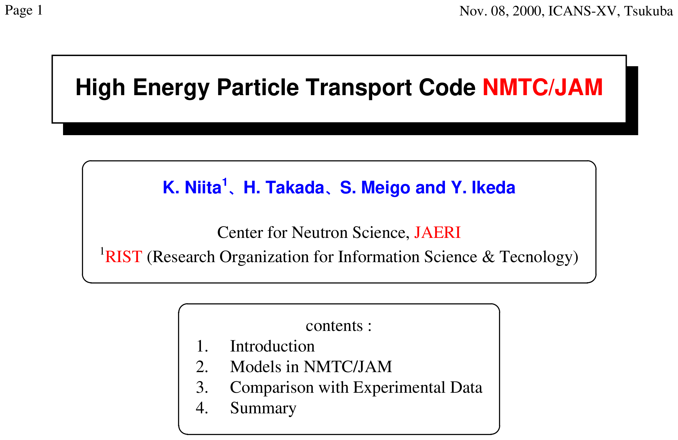
Fig. 3.1 Slide 1

3.1.2. Slide 2

It is convenient if the slides of one presentation are in one file. You can also make a slide show by turning the pages when displaying images from your computer and making a presentation. ANGEL uses multi-page. The following example is on page 2.

List 3.2 • Slide 2

 1:  newpage:
 2:  p: secl notf bfon(5)
 3:  set: c1[12] c2[16]
 4:
 5:  w:Page \page/ x(-2) ix(1) y[c2+1] iy(1)
 6:  w:Nov. 08, 2000, ICANS-XV, Tsukuba/ x(26) ix(3) y[c2+1] iy(1)
 7:
 8:  wt: x(1) ix(1) y[c2-0.5] iy(2) s(1.2) box(ShadowBox) c(e) f(7)
 9:  Introduction
10:  e:
11:
12:  ab: x(10) y[c2-1] ax(10) ay[c2-14] a(1.8) c(e) cb(y)
13:
14:  wt: x(8) ix(1) y[c2-0.5] iy(3) s(1.0) box(OvalBox) b(1.2)
15:  {\hv\bf\large{\color{b}NMTC/JAERI97} + {\hv\bf\color{b}MCNP4A}}
16:  e:
17:
18:  wt: x(2) ix(1) y[c2-2.7] iy(3) box(OvalBox) b(1.2)
19:  Joint Project of JAERI and KEK, high intensity proton \
20:  {\color{r} 600 MeV - 50 GeV}
21:  Neutronics optimization study of the high intense Spallation Neutron Source
22:  ASTE (AGS Spallation Target Experiment) {\color{r} 1.5 - 24 GeV}
23:  e:
24:
25:  wt: x(6) ix(1) y[c2-6.5] iy(3) box(OvalBox) b(1.2)
26:  High Energy Nuclear Reactions
27:  Many kinds of transport particles in additin to the nucleons and pions
28:  e:
29:
30:  wt: x(8) ix(1) y[c2-9.5] iy(3) s(1.0) box(OvalBox) b(1.2)
31:  Limit of Bertini model
32:  only nucleon and pion
33:  upper limit: {\color{b}3.5 GeV} for nucleons and {\color{b}2.5 GeV} for pions
34:  e:
35:
36:  wt: x(10) ix(2) y[c2-14] iy(3) box(OvalBox) b(1.2)
37:  High Energy Particle Transport Code
38:
39:  {\hv\bf\Large{\color{b}NMTC/JAM}}
40:  e:

The first line is the declaration of the new page. The yellow hollow arrow is drawn on the 12th line. The shape is drawn before the comment, so this long arrow is partially hidden by the comment box.

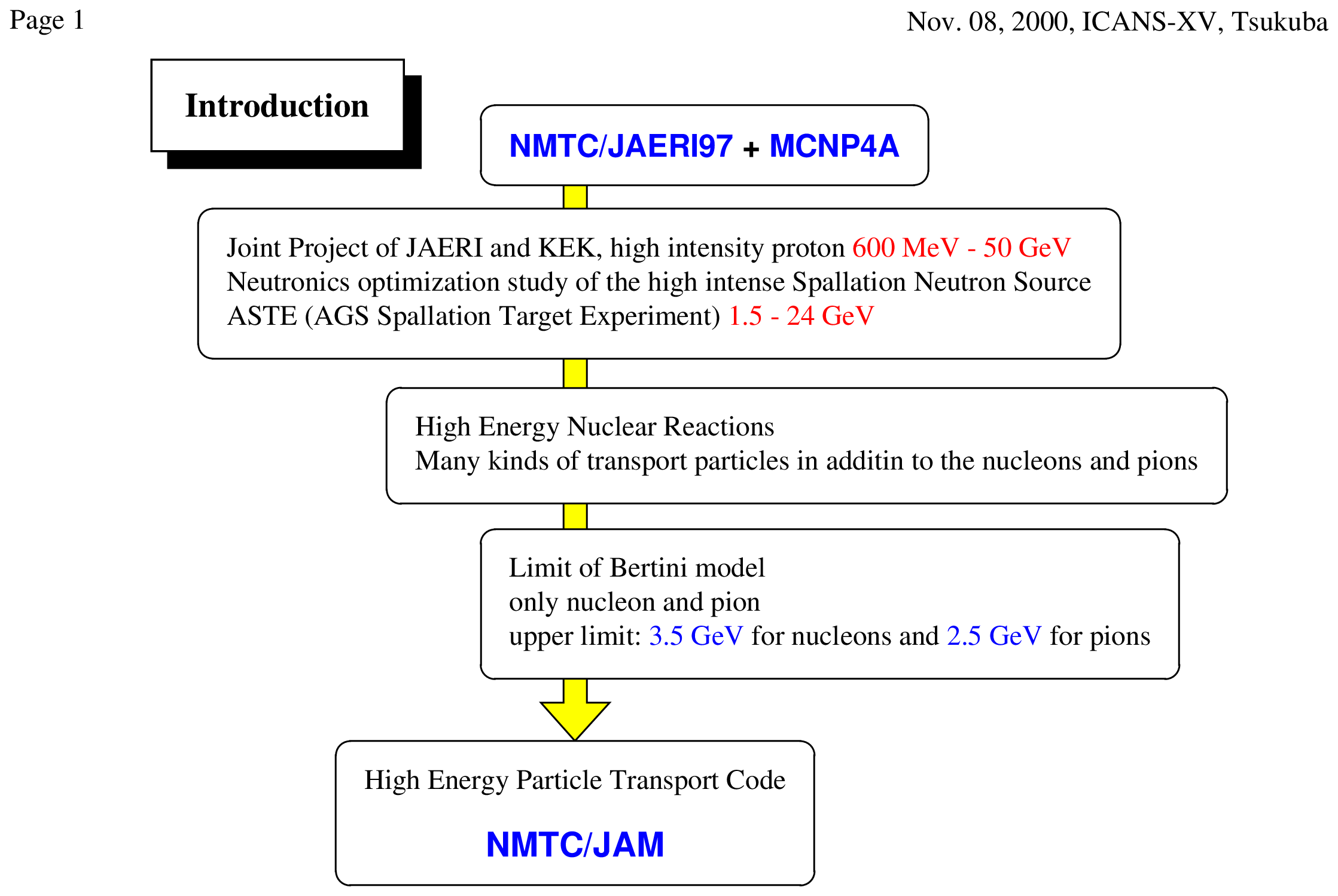
Fig. 3.2 Slide 2

3.1.3. Slide 3

This is the third page.

List 3.3 • Slide 3

 1:  newpage:
 2:  p: secl notf bfon(5)
 3:  set: c1[12] c2[16] c3[0.0] c4[14.5]
 4:
 5:  w:Page \page/ x(-2) ix(1) y[c2+1] iy(1)
 6:  w:Nov. 08, 2000, ICANS-XV, Tsukuba/ x(26) ix(3) y[c2+1] iy(1)
 7:
 8:  h: ny3 x=[y3+c3] ny1 y2=[-y1+c4+0.7],l0tt
 9:   4   2
10:   4   0
11:  10   0
12:
13:  wt: x[c3+9.0] ix(1) y[c4+0.7] iy(2) s(1.2) box(OvalBox) c(e) f(1)
14:  {\color{r}J}et {\color{r}A}A {\color{r}M}icroscopic Transport Model
15:  e:
16:
17:  wt: x[c3+12] ix(2) y[c4-1.3] iy(3) s(1.3) box(OvalBox) b(1.7)
18:  is a &{\SingleBox{e}{w}{r}\hv\it Hadronic Cascade Model}  ,
19:  \vspace{0.5}\
20:  which explicitly treats &{\Singlebox{e}{y}{y}all established hadronic states}
21:  including &{\Singlebox{e}{y}{y}resonances} with explicit spin and isospin
22:  as well as their &{\Singlebox{e}{y}{y}anti-particles}.
23:  e:
24:
25:  wt: x[c3+1.8] ix(1) y[c4-1.7] iy(2) s(1.3) box(shadowBox) cb(r)
26:  {\hv\bf\Huge{\color{y}JAM}}
27:  e:
28:
29:  wt: x[c3+4.5] ix(1) y[c4-9.5] iy(3) s(1.3) box(OvalBox) b(1.7)
30:  We have parametrized
31:  {\Singlebox{e}{y}{y}\
32:  all {\color{r}H}adron-{\color{r}H}adron Cross Sections}
33:  based on the {\SingleBox{e}{w}{r}\hv\it Resonance model} and \
34:  {\SingleBox{e}{w}{r}\hv\it String model}
35:  by fitting the available experimental data.
36:  e:
37:
38:  wt: x[c3+14.8] ix(1) y[c4-7.1] iy(3) s(1.0) box(OvalBox) b(1.7) c(b)
39:  119 kinds of Mesons
40:  170 kinds of Baryons
41:  e:

Lines 8-11 draw a line connecting the comments. Comments are drawn in the order written in the input, so take that into account when stacking. It may seem a little complicated, but it is not difficult to write more sentences first and then add decorations in sequence.

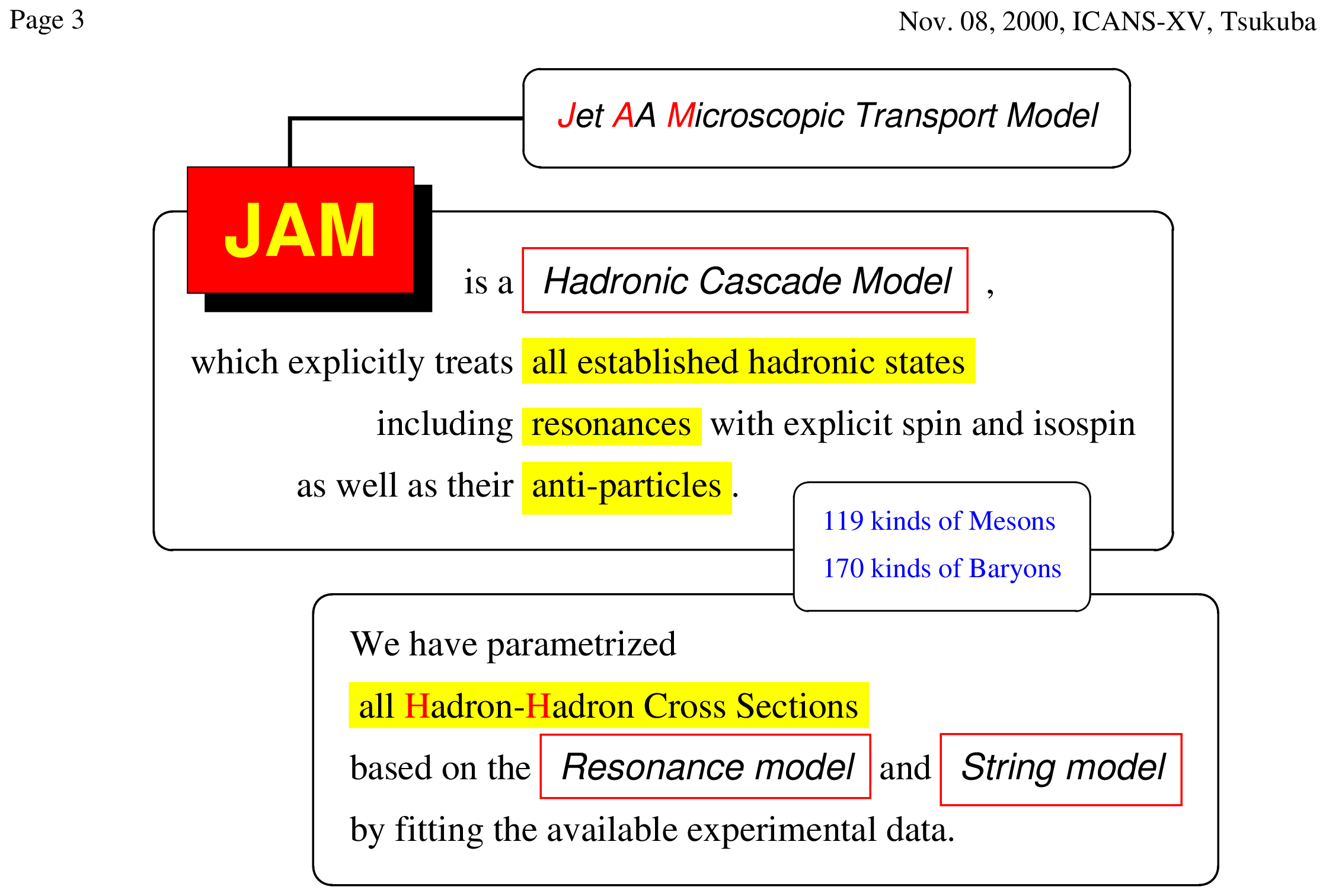
Fig. 3.3 Slide 3

3.1.4. Slide 4

This is the 4th page. Next, the graph will finally be included.

List 3.4 • Slide 4

 1:  newpage:
 2:  p: secl notf bfon(5)
 3:  set: c1[12] c2[16]
 4:
 5:  w:Page \page/ x(-2) ix(1) y[c2+1] iy(1)
 6:  w:Nov. 08, 2000, ICANS-XV, Tsukuba/ x(26) ix(3) y[c2+1] iy(1)
 7:
 8:  wt: x[c1+3] ix(2) y[c2-1] iy(2) s(1.4) box(Shadowbox) c(e) f(1)
 9:  {\color{r}P}roton-{\color{r}P}roton\
10:   {\color{r}I}nelastic Cross Section
11:  e:
12:
13:  z: xorg(0.33) yorg(0.14)
14:
15:  p: xmax(10) ymax(60) ymin(0) xmin(1) nosp
16:
17:  x:E_{cm} (GeV)
18:  y:\sigma (mb)
19:
20:  a: x(-1.5) y(0) ax(2.1) ay(10) t c(b)
21:
22:  p: legs(1.0) legx(-4.3) legy(10) lbox(Shadowbox) lbcb(y) lbcl(e)
23:
24:  w:total/ x(6.5) y(42) s(1.4)
25:  w:inelastic/x(4.3) y(32) s(1.4) c(j)
26:  w:String/x(5) y(20) s(1.4) c(r) a(17)
27:  w:Resonance/ x(6) y(11) s(1.4) c(b) a(-8)
28:
29:  h:  ny1  x  y2,n4xx  ny3  dy2
30:  infl: {pp_tot.exp}
31:  h: x ny1 y2,l0 n n n n
32:  infl: {pptot.dat}
33:  h: n x y1,lt0b  y2,ltt0j y3,lt0r
34:  infl: {ppinel.fit}
35:  h: n x y1,i0y  ny2,l0 ny3,lt0rrr
36:  infl: {ppinel.fit}
37:  h: n x y(NN \to  N\Delta\(1232\)),d0b
38:  infl: {pp-nd.fit}
39:  h: n x y(NN \to  NN^*),d0
40:  infl: {pp-nns.fit}
41:  h: n x y(NN \to  N\Delta^*),u0rr
42:  infl: {pp-nds.fit}
43:  h: n x y(NN \to  RR),m0
44:  infl: {pp-rr.fit}

After writing the title of the graph on lines 8-11, it becomes the section of the multigraph on lines 13. Now move from the SECL graph axis to the next graph axis. The origin of the new axes is defined by xorg(0.33) yorg(0.17).

In the new graph, lines 29-44 draw experimental points, fitted lines, etc. while reading data from other files. At that time, a figure legend is written.

The display position of the figure legend has been moved from the default position using the parameters on line 22. At the same time, it is surrounded by a box using lbox.

The meaning of each line is written on the graph in the comment line on the 24-27th line. On line 27, the opponent’s line is tilted, so the comments are also tilted a little accordingly.

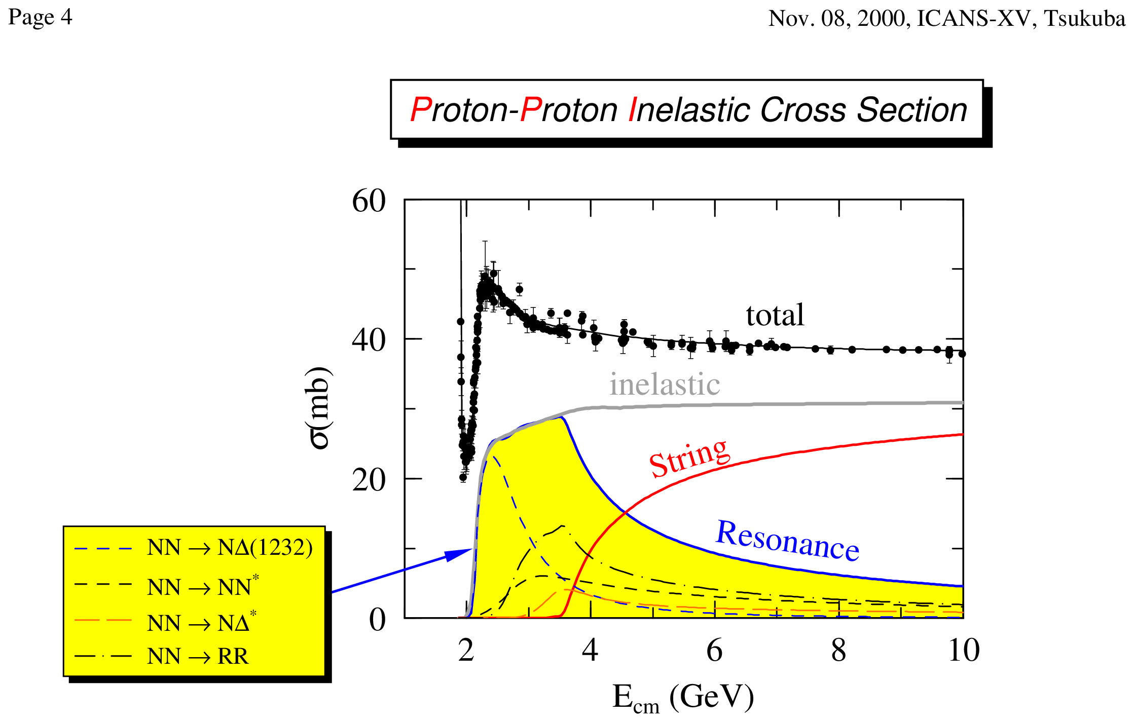
Fig. 3.4 Slide 4

3.1.5. Slide 5

This is the 5th page. Next, there are two graphs.

List 3.5 • Slide 5

 1:  newpage:
 2:  p: secl notf bfon(5)
 3:  set: c1[12] c2[16]
 4:
 5:  w:Page \page/ x(-2) ix(1) y[c2+1] iy(1)
 6:  w:Nov. 08, 2000, ICANS-XV, Tsukuba/ x(26) ix(3) y[c2+1] iy(1)
 7:
 8:  wt: x[c1] ix(2) y[c2-1] iy(2) s(1.2) box(ShadowBox) c(e) f(1)
 9:  {\color{r}N}ucleon-{\color{r}N}ucleus {\color{r}D}ifferential \
10:  {\color{r}E}lastic Cross Sections
11:  e:
12:
13:  z:
14:  infl: {pb208ne.ang}
15:  p: xorg(0.12) yorg(0.0) scal(0.5)
16:
17:  z:
18:  infl: {pb208nd.ang}
19:  p: xorg(1.2) yorg(0.0) scal(1.0) noyt

Here, two files are read in lines 13-15 and 17-19, and two graphs are drawn. In the file to be read, scal, xorg, yorg etc. are already defined in order to format it as an input of ANGEL , so redefine the values of these parameters after reading the file.

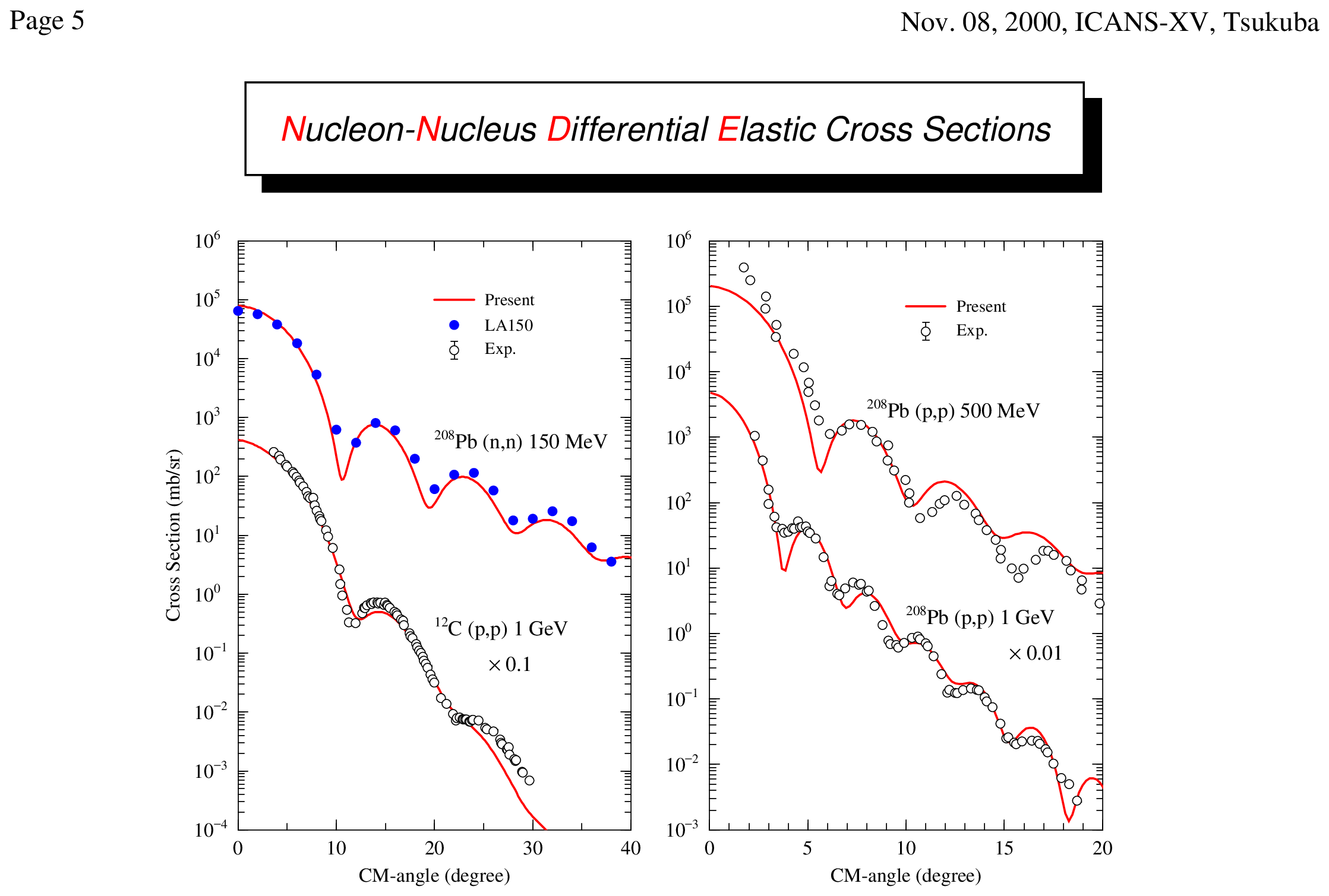
Fig. 3.5 Slide 5

3.1.6. Slide 6

This is the 6th page. Next, a handwritten figure is written together with the text.

List 3.6 • Slide 6

 1:  newpage:
 2:  p: secl notf bfon(5)
 3:  set: c1[12] c2[16]
 4:
 5:  w:Page \page/ x(-2) ix(1) y[c2+1] iy(1)
 6:  w:Nov. 08, 2000, ICANS-XV, Tsukuba/ x(26) ix(3) y[c2+1] iy(1)
 7:
 8:  wt: x[c1] ix(2) y[c2-2] iy(2) s(1.2) box(ShadowBox) c(e) f(1)
 9:  Comparison with Experimental Data (3)
10:  e:
11:  wt: x(3) y[c2-5] f(0) box(ovalBox)
12:  (3)  & Reaction rate distribution on Mercury target (AGS)
13:       & \H. Takada, et.al, Proc. of the 14th Mtg. of the Int. Collaboration on\
14:       & \Advanced Neutron Sources, Illinois, 1998, Vol.II\
15:       & TARGET：    Hg cylinder,   diameter 20 cm,  length 130 cm
16:       & ENERGY：    Proton   1.6, 12, 24 GeV
17:       & DETECTOR：  Activation detector (In, Bi, Co, Ni, Al, Nb)
18:  e:
19:
20:  set: c3[3] c4[-3]
21:
22:  w: Hg Target/x[11+c3] ix(2) y[5+c4] iy(2) s(1.0)
23:  polg: pl(0) x[5+c3] y[5+c4] s(1.1) cl(o) cb(o)
24:  h: v=[0.5,1.5,100] x=[5+c3+cos(v*pi)] y=[5+c4+sin(v*pi)],l0tt
25:  h: x+3 y-3,n0io
26:   5 6
27:  18 6
28:  18 4
29:   5 4
30:   5 6
31:  h: x+3 y-3,l0tt
32:   5 6
33:  18 6
34:  18 4
35:   5 4
36:
37:  aw:samples/x[12+c3] y[2+c4] ax[10+c3] ay[3.5+c4]
38:  h: x+3 y-3,iy
39:   4 3.9
40:  18 3.9
41:  18 3.5
42:   4 3.5
43:   4 3.9
44:  h: x+3 y-3,l0
45:   4 3.9
46:  18 3.9
47:  18 3.5
48:   4 3.5
49:   4 3.9
50:
51:  wt: x[-2+c3] y[4.7+c4]
52:  &proton beam
53:  1.6, &12, 24 GeV
54:  e:
55:  a: x[-2+c3] y[5+c4] ax[3.5+c3] ay[5+c4] t
56:  h: x+3 y-3,l0
57:   4 7
58:   4 4
59:  h: x+3 y-3,l0
60:  18 7
61:  18 3
62:  h: x+3 y-3,l0
63:   2 6
64:  20 6
65:  h: x+3 y-3,l0
66:   2 4
67:  20 4
68:  a: x[19+c3] y[7+c4] ax[19+c3] ay[6+c4]
69:  a: x[19+c3] y[3+c4] ax[19+c3] ay[4+c4]
70:  w:20 cm/x[18.5+c3] y[5+c4] iy(2)
71:  a: x[ 8+c3] y[6.5+c4] ax[ 4+c3] ay[6.5+c4]
72:  a: x[14+c3] y[6.5+c4] ax[18+c3] ay[6.5+c4]
73:  w:130 cm/x[11+c3] y[6.5+c4] iy(2) ix(2)

Lines 22-35 draw the gray part of Hg Target. Line 23 fills the circle with polg, and the next line 24 uses self-running variables and column functions to draw the perimeter of the semicircle.

Use lines 25-30 to gray the rectangle and lines 31-35 to outline the perimeter.

Lines 38-49 present the yellow part. After these lines, arrows, lines, and dimensions are described. It is a little troublesome, but it is not difficult because you can decide the coordinates while looking at the graph paper. I define constants just in case I need to move the whole thing after I finish writing.

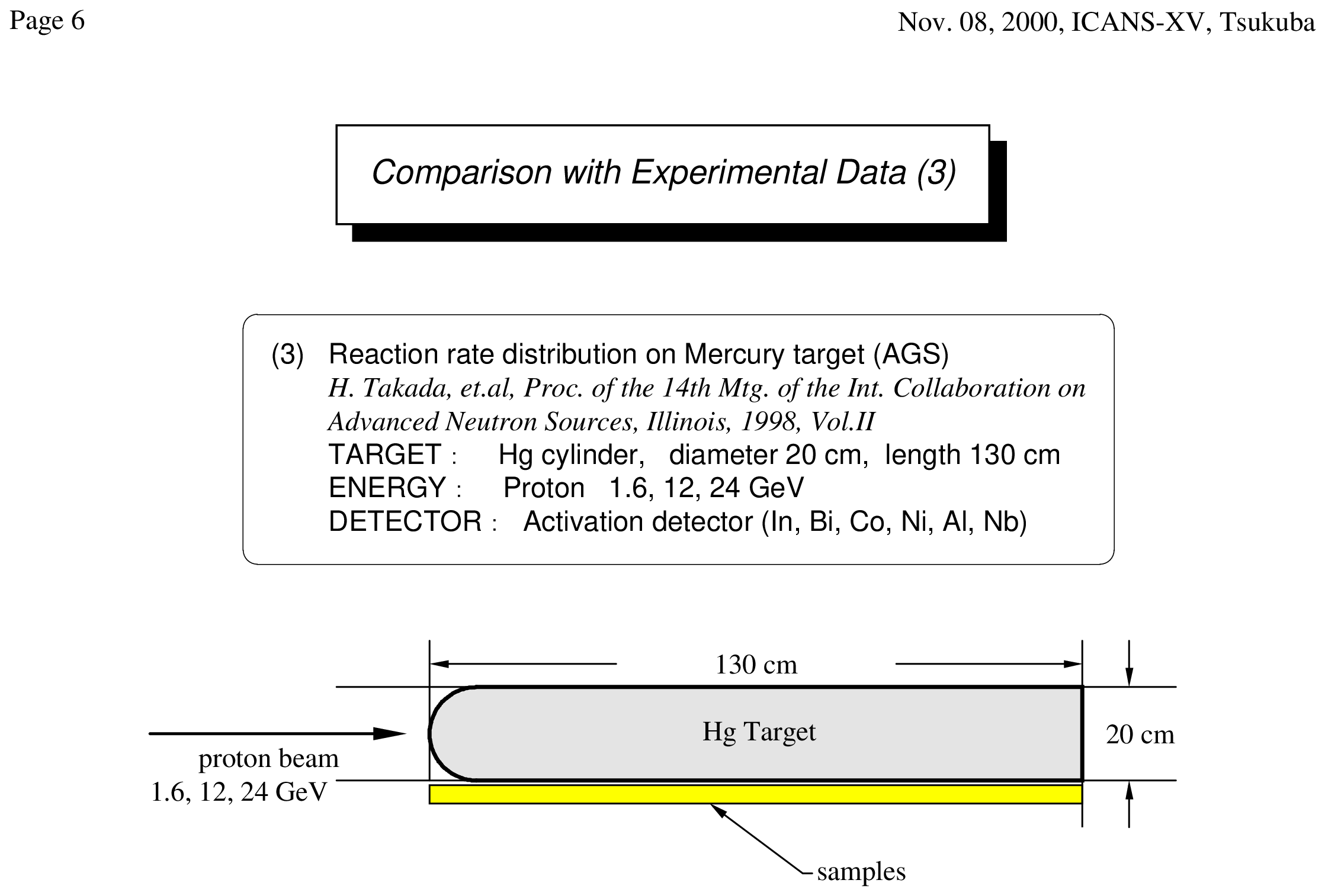
Fig. 3.6 Slide 6