4.12. Example: Comprehensive DCHAIN-PHITS calculation
This example seeks to highlight some of the various features within DCHAIN. The PHITS input deck located at <PHITS-install>/dchain-sp/sample/simple/phits_simple.inp and also shown in Appendix 6.1 was used to generate the input files for DCHAIN automatically. The simulation consists of a 1 cm diameter pencil beam of 250 MeV protons incident on a cylindrical rod composed of three segments: tungsten, water, and iron. This rod is surrounded by beryllium on the side and back. This structure is irradiated with a beam current of 100 nA for 6 minutes, reduced to 50% power (50 nA) for 4 minutes, and then left to cool for 50 minutes. Temporarily changing the icntl PHITS input parameter to icntl= 8, the geometry can be visualized as shown in Figure 4.12.1.
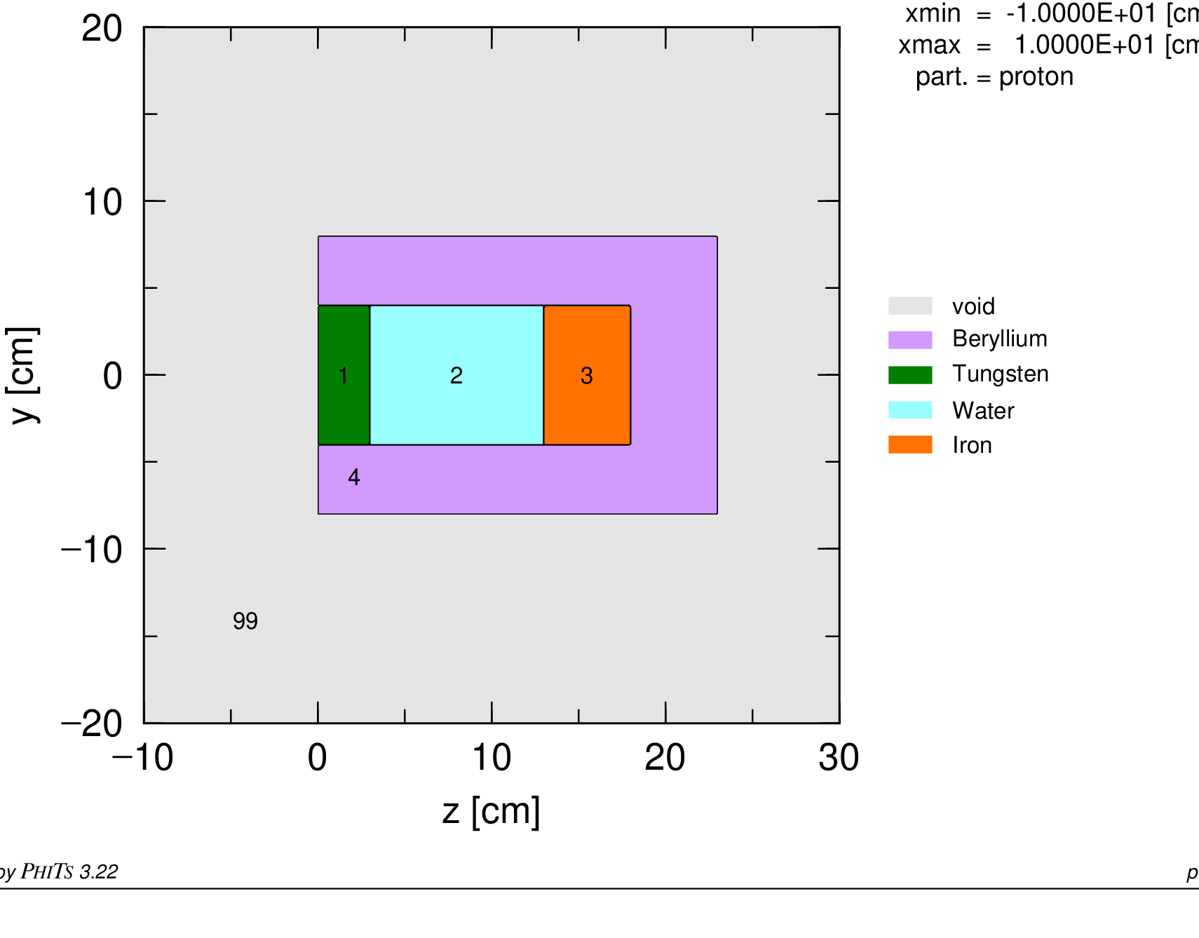
Fig. 4.12.1 PHITS geometry of example case (see: yz-track_geo.eps)
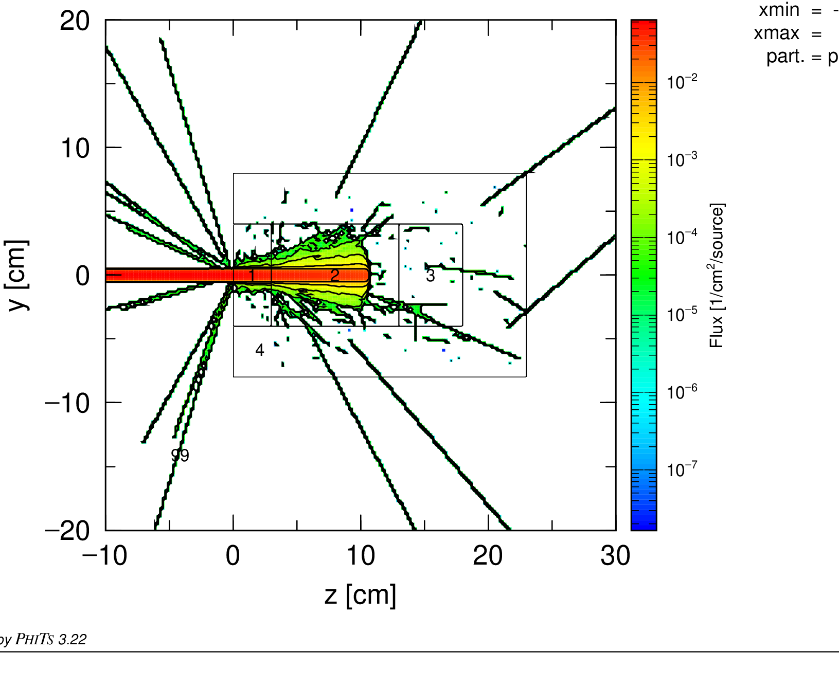
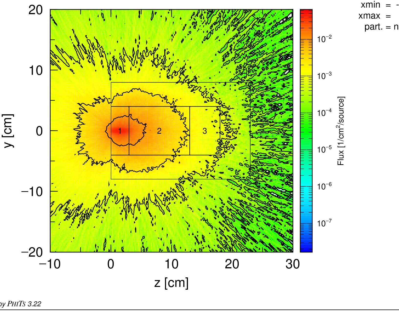
This example seeks to highlight both spallation-driven activation (in the tungsten portion) as well as neutron reaction-driven activation (in the iron portion). Resetting it to icntl= 0 and rerunning the PHITS simulation in its normal mode, the proton and neutron flux distributions within the geometry can be visualized as shown in Figures 4.12.2–4.12.3. Note that the proton beam ranges out in the water portion of the volume.
This generates a file called “spallation.out” (as specified by file in [T-Dchain]), which is shown in Appendix 6.2, in addition to the support files “spallation.dtrk” (containing neutron fluxes), “spallation.dyld” (containing nuclide yields from everything except neutrons under 20 MeV), and “dch_link.dat” (which simply passes the file path to DCHAIN’s data library folder). Note that if using the older full format (iredufmt= 0) rather than the new reduced format (iredufmt= 1, default) when running PHITS an additional file called “spallation_err.dyld” would had been generated, containing the uncertainties associated with the nuclide yields.
This file can then be ran through DCHAIN without any modifications. All of the resulting files will named “spallation.*” with various extensions; explanations of each of these will be given here. Providing immediate visualization of results, when executing DCHAIN in the suggested default manner (via the batch/shell scripts), ANGEL is automatically ran after DCHAIN and produces time-dependent plots of the activity, decay heats, and more; the activity plot is shown in Figure 4.12.4. This is from the “spallation.eps” file which is generated from the “spallation.ang” ANGEL input file; this ANGEL input file can be manipulated and reran through ANGEL if wishing to make any modifications to the plots. We can see in this figure that during the irradiation process that the Be region (cell 4) is responsible for much of this activity, but it rapidly drops off to a comparatively negligible level after the end of the irradiation period.
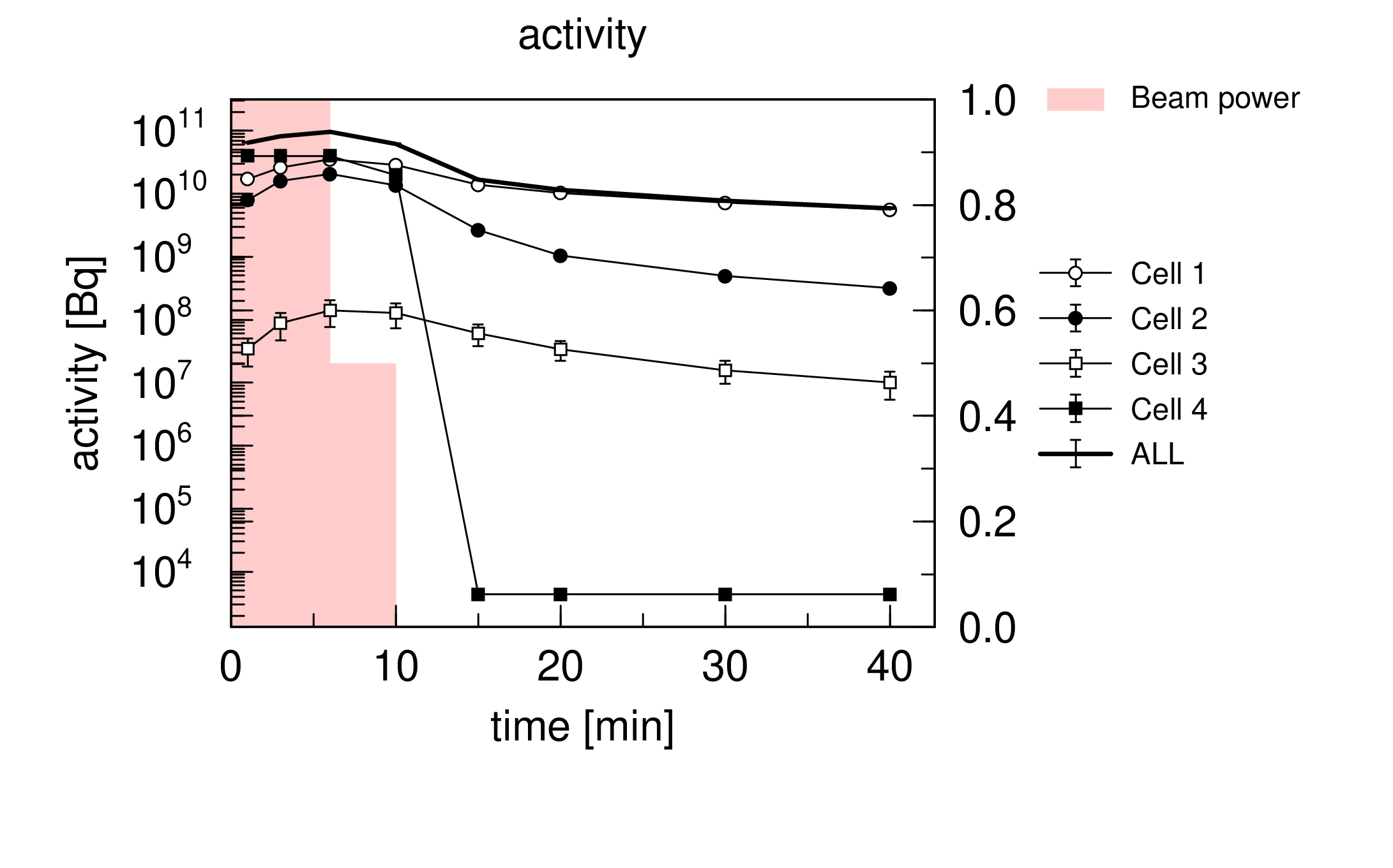
Fig. 4.12.4 Time-dependent activity in each region (generated with ANGEL).
At the bottom of the DCHAIN input file is a set of parameters controlling what is written to the *.ang file. Of particular note, IANGBPWR controls whether the beam power schedule is overlaid on the plots (the shaded red area in the figure), ANGELOUT_REGION controls for which regions output data is written, and ANGELOUT_NUCLIDES allows for specification of individual nuclides to plot along with the region-wise data. For instance, if we wanted to just look at a few nuclides (say, \(^{56}\)Mn, \(^{53}\)Fe, and \(^{53m}\)Fe) in the region made of iron (cell 3), ignoring the activity elsewhere, this bottom section of parameters could be modified as shown below, producing the plot shown in Figure 4.12.5.
angelout_region     = 3
angelout_nuclides   = 3
   Mn-56
   Fe-53
   Fe-53m
Here, the output specified by ANGELOUT_NUCLIDES represents the sum over the regions defined by reg= in [t-dchain], and is different from the regions specified by ANGELOUT_REGION.
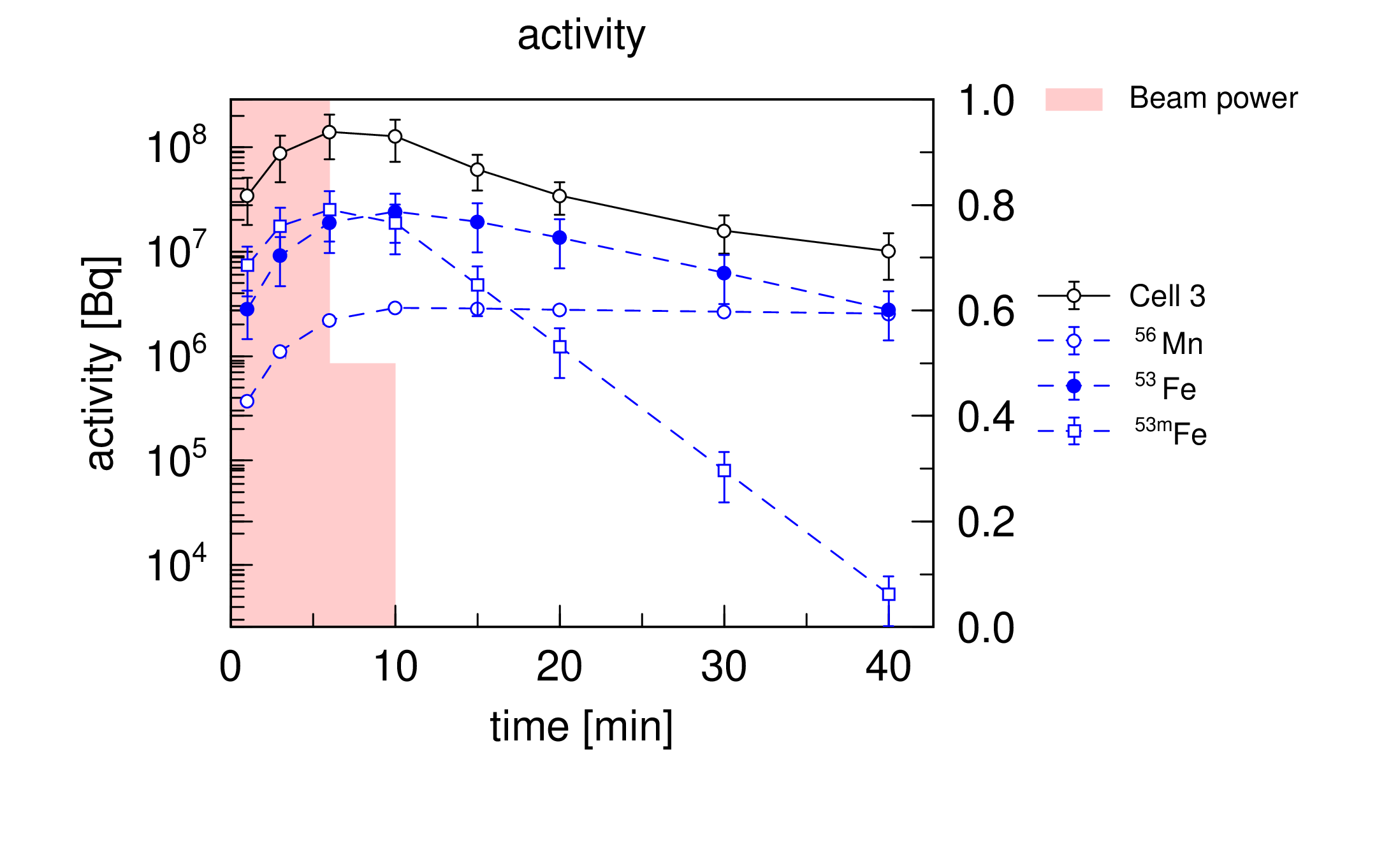
Fig. 4.12.5 Time-dependent activity in region 3 with specific nuclides featured.
The primary output file containing more detailed information ends with the “*.act” extension (“spallation.act” here). In this file, we can survey the exact inventories, activities, decay heats, photon spectra, etc. in each region and at each time step. However, one may note that for this example that the file is quite lengthy and that many of the nuclides listed only contribute negligibly to the total activity. The activity threshold for what nuclides are printed to this file is controlled by the ACMIN parameter, and PHITS sets this value to \(10^{-20}\) by default, meaning it includes all nuclides with at least \(10^{-20}\) Bq of activity, an extremely tiny threshold which usually results in inclusion of essentially every nuclide produced. While the “Top 10” sections within the file isolate the 10 most important nuclides for activity, decay heat, and photon dose, one may wish to view the entire file with the less significant nuclides omitted. Here, we can adjust this parameter to a new value of ACMIN= -1.0E+4, meaning any nuclides with at least \(10^4\) atoms/cm\(^3\) are included. While the tungsten section remains somewhat lengthy due the large variety of spallation products with relatively similar yields, the iron section (region 3) is notably reduced by some of the very obscure nuclides (produced through very rare neutron reactions) now being excluded, taking the total number of nuclides reported at t=1 minute from 45 down to 17. If using the unofficial Python “DCHAIN Tools” package for parsing this file (demonstrated later), this length concern is likely not particularly important except for substantially large geometries (or in cases with many output times) where space conservation is a general concern.
Somewhat similar to the “Top 10” sections of the *.act file, the “spallation.alr” file reports the top 30 nuclides contributing to the total activity and total decay heat integrated over all regions at each requested output time outtime/ITOUT. Also, the “spallation.yld” file prints the final inventories of each nuclide (making up a fractional contribution at least \(10^{-12}\) of the total atoms per unit volume) in each region. The IYILD parameter controls whether this total does (default) or does not include the original target nuclide inventories.
The DCS (decay chain scheme) file, “spallation.dcs” here, contains information regarding how the inventory of each nuclide changes with each time step. By default, it only shows change in inventory and the decay chain scheme responsible for that change. Detailed information on the contribution from each link in each chain (and whether it is from high-energy reactions or neutron reactions/decay) can be made visible by setting IWRCHDT= 1 (default 0). Additionally, in irradiation periods only the change occurring in the final of IDIVS substeps is printed by default; setting IWRCHSS= 1 (default 0) prints the changes occurring in every single irradiation substep too. Both of these features (especially IWRCHSS= 1) make the DCS output file quite notably larger; however, together they allow for exact tracking of what reactions are responsible for every change in inventory calculated by DCHAIN. The CHRLVTH parameter can be used to tune how big an inventory change from a single decay/reaction chain must be to warrant being written to the DCS file. Also, since one is often only concerned with this level of detailed tracking for specific nuclides, the advanced option IWRCHNUC allows for specific tracking of only listed nuclides of concern.
Relating to this example, the portion of the DCHAIN input file controlling the DCS file could be changed as shown below to display only the decay chains relevant to the production of the eight listed nuclides made in the iron volume (region 3) and to show detailed information on which links of each chain are contributing to their inventories. Note that IWRCHSS= 0 has been left unchanged; the last substep usually provides a sufficient idea of the relative contribution of each link in each chain. Setting IWRCHSS= 1 is usually only necessary if target nuclide inventories are expected to notably change over an irradiation time step or if complete tracking of all inventory changes is desired.
iwrtchn =       1
chrlvth = -1.0000E+00
iwrchdt =       1  ! write more detailed information on each link in decay chain file
iwrchss =       0
! add special "iwrchnuc" parameter for tracking of specific nuclides in this DCS file
iwrchnuc =      8
      Cr-49
      Mn-56
      Fe-53
      Cr-55
      Cr-51
      V-48
      Mn-54
      Fe-55
Upon running this updated input deck, note the absence of nuclides listed in the other three regions (which don’t contain those listed nuclides at all) and the three extra lines appearing between each decay chain scheme outlining the different production mechanisms for each nuclide. This highlights that while DCHAIN prints the full decay chains that it constructs, in most cases only the last few links of a chain really contribute a noteworthy amount to the inventory of each nuclide of interest.
The “spallation.pht” file contains PHITS-formatted [Source] sections for the photon spectrum in each region at each time step. Note that, if it is more convenient (such as if using the PHITS insert file “infl:” functionality), one may choose to output this file individually at each requested time step rather than all in one file by adjusting the PHITSOUT input parameter from 1 to 2. This functionality is useful for performing secondary dose assessments for an activated object/area as a function of cooling time and/or shielding configuration. As a caveat though, do keep in mind that the spatial distribution of activation is considered to be homogeneous throughout each individual region, an assumption which can be quite poor for large regions. Thus, if wishing to perform these secondary assessments, please ensure this is taken into account when designing the tally regions. Subdivision into smaller regions or use of an xyz mesh would provide better spatial resolution where needed.
As somewhat legacy features, the “spallation.gsd” file contains similar MCNP-formatted SDEF (source definition) cards with the photon spectrum for each region and at each time step, and the “spallation.gso” file describes the nuclides present in each photon spectrum energy group and their relative contributions to them for each region and output time.
The “spallation.mat” file contains PHITS-formatted [Material] sections (material cards also compatible with MCNP) for each region and output time step. Similar to the PHITS-formatted [Source] sections, these are by default outputted into a single file but can be separated by time step with the IMTCARD parameter. While DCHAIN does approximate the effects of target burnup (reduced production rates of nuclides through spallation of the target nuclides being depleted), it is still ultimately an approximation. For the most accurate results, an iterative calculation involving cycling between PHITS and DCHAIN calculations numerous times is necessary. Though in most simulations the composition of the materials is not changed enough to make this effect even noticeable, some simulations do observe notable changes in material composition. While this is unlikely to be especially significant for a majority of simulations involving just high-energy reactions, it can be quite notable in neutron-driven environments if there is a buildup of nuclides which would affect the neutron flux spectrum (which DCHAIN takes to be constant). Thus, this feature plays an important role in simplifying iterative DCHAIN and PHITS burnup calculations where the neutron flux is expected to change with time. See Card 4 for more information on customization involved with this functionality.
The “spallation.lst” file is just where most of the terminal output printed during DCHAIN’s execution is rerouted to. This file contains the input echo from DCHAIN, explanations of all input parameters, warning messages, and diagnostic information.
The DCHAIN Tools module is useful for quickly parsing DCHAIN output. It is now available as a submodule of PHITS Tools, for which installation with pip install PHITS-Tools is recommended. See the DCHAIN Tools documentation for details; the original repository also provides a short PDF manual and summary of the output dictionary structure. Below is a short Python script using the module to parse this example’s DCHAIN output and survey some of the results. The terminal output observed from running this script is also included below.
from dchain_tools import *
import numpy as np
import matplotlib.pyplot as plt

# path to the folder containing output files
simulation_folder_path = r'C:\phits\lecture\advanced\DCHAIN3\\'
# the filename part before the extension of all of the output files
simulation_base_name = 'spallation'

# Provide this path information to the main DCHAIN parsing function
# It parses *.act and, if found, *.dtrk and *.dyld too (and *.dcs if enabled).
dchain_output = process_dchain_simulation_output(simulation_folder_path,simulation_base_name,process_DCS_file=False)

# Output can be accessed in 'dictionary' or 'class/attribute' styles.
# print list of all nuclides (as text strings) found in the second region over all times
print(dchain_output['nuclides']['names'][1]) # dictionary-style access
# print total activity and its absolute error in the second region and first time step
print (dchain_output.nuclides.total.activity.value[1][0], dchain_output.nuclides.total.activity.error[1][0]) # attribute-style access

# find the activity of Fe53 in the 3rd region at the 5th time step
ri = 2   # region index
ti = 4   # time index
# get desired nuclide name string formatted in DCHAIN's specific 6-character syntax
Fe53_Dname = nuclide_plain_str_to_Dname('Fe-53')
# determine index of desired nuclide among all nuclides in this region
Fe53_index = dchain_output['nuclides']['names'][ri].index(Fe53_Dname)
# now extract the activity value
A_Fe53 = dchain_output.nuclides.activity.value[ri][ti,Fe53_index]
print('A(Fe-53) in [Bq/cc] in region 3 at 5th output time: ',A_Fe53)
Parsing DCHAIN activation file...                  (0.01 seconds elapsed)
    Restructuring nuclide data table array...          (0.05 seconds elapsed)
['H   3 ', 'He  6 ', 'Li  5 ', 'Li  8 ', 'Li  9 ', 'Be  7 ', 'Be  8 ', 'Be 10 ', 'Be 11 ', 'B   8 ', 'B   9 ', 'B  12 ', 'B  13 ', 'C  10 ', 'C  11 ', 'C  14 ', 'C  15 ', 'N  13 ', 'N  16 ', 'N  17 ', 'N  18 ', 'O  14 ', 'O  15 ', 'O  19 ', 'Hf178n', 'Re188 ', 'Re188m']
15921500.0 563170.0
A(Fe-53) in [Bq/cc] in region 3 at 5th output time:  76742.0
As a very quick aside, one may notice the inclusion of the second metastable state of \(^{178}\)Hf and two \(^{188}\)Re isomers in this list of present nuclides in region 2 (which is composed of water). This is not a bug; indeed, these nuclides are present in both the DCHAIN output and in the *.dyld file generated by PHITS. The [T-Yield] tally automatically invoked by [T-Dchain] uses the setting output= cutoff rather than the default behavior of output= product, tallying each particle/nucleus in the cell in which its history ends, not where it was spawned, since this is ultimately what is needed for activation calculations. This is generally more important for lighter particles like tritons, though, as in this case, heavier recoil products near a cell boundary may drift from one cell to another.
Once imported in Python, the results can also be quite easily visualized. Figures 4.12.6–4.12.7 show a re-creation of the activity plot generated by ANGEL from earlier and a plot of the photon spectrum in the first region at the end of the irradiation period. The code added to the Python script for generating these plots is also shown below.
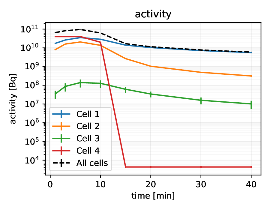
Fig. 4.12.6 Time-dependent activity in each region (generated with Python).
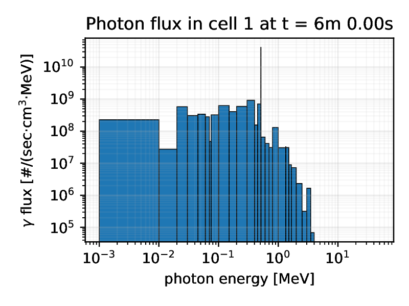
Fig. 4.12.7 Cell 1 photon flux right after end of irradiation at t = 6 mins
# Recreate ANGEL activity plot
plt.figure(0,(4.5,3.5)) # figure index and dimensions
t_minutes = np.array(dchain_output.time.from_start_sec)/60
total_activity , total_activity_error = 0 , 0
for ri in range(len(dchain_output.region.numbers)): # for each region
    region_volume = dchain_output.region.volume[ri]
    plt.errorbar(t_minutes,
                 dchain_output.nuclides.total.activity.value[ri][:]*region_volume,
                 dchain_output.nuclides.total.activity.error[ri][:]*region_volume,
                 label='Cell {}'.format(ri+1))
    total_activity += dchain_output.nuclides.total.activity.value[ri][:]*region_volume
    total_activity_error += (dchain_output.nuclides.total.activity.error[ri][:]*region_volume)**2
total_activity_error = total_activity_error**0.5
# Total activity line
plt.errorbar(t_minutes,total_activity,total_activity_error,
             label='All cells',linestyle='--',color='k')
plt.yscale('log')
plt.legend(loc='best')
plt.xlabel('time [min]')
plt.ylabel('activity [Bq]')
plt.title('activity')
plt.grid(b=True, which='major', linestyle='-', alpha=0.25)
plt.grid(b=True, which='minor', linestyle='-', alpha=0.10)
plt.tight_layout()

# Plot photon spectrum in region 1 at 3rd time step
# Note: as in the *.act file, photon spectra are binned by energy in descending order
plt.figure(1,(4,3)) # figure index and dimensions
bin_widths = dchain_output.gamma.spectra.E_upper[0][2,:]-dchain_output.gamma.spectra.E_lower[0][2,:]
plt.bar(x=dchain_output.gamma.spectra.E_lower[0][2,:],align='edge',
        width=bin_widths,
        height=dchain_output.gamma.spectra.flux.value[0][2,:]/bin_widths,
        edgecolor='k',linewidth=0.5)
plt.xscale('log')
plt.yscale('log')
plt.xlabel('photon energy [MeV]')
plt.ylabel(r'$\gamma$ flux [#/(sec$\cdot$cm$^3$$\cdot$MeV)]')
plt.title('Photon flux in cell 1 at t = {}'.format(seconds_to_dhms(dchain_output.time.from_start_sec[2])))
plt.grid(b=True, which='major', linestyle='-', alpha=0.25)
plt.grid(b=True, which='minor', linestyle='-', alpha=0.10)
plt.tight_layout()

plt.show()
And, serving mostly to conveniently and quickly assess important nuclides as a function of time and/or region, the DCHAIN Tools package also has a function suited for automatically generating plots ranking nuclides as shown below in Figure 4.12.8.
plot_top10_nuclides(dchain_output,region_indices=2)
plt.show()
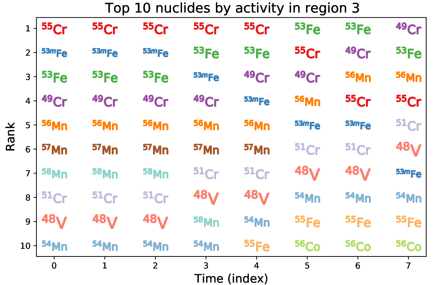
Fig. 4.12.8 Ranking of nuclides by activity in region 3 as a function of time index.
One of the relatively new features in DCHAIN is the ability to choose among a variety of decay and neutron reaction cross section libraries. If one wishes to change the cross section library used for neutron reactions under 20 MeV, only the INXSLIB parameter must be changed, and that will be demonstrated here by comparing the final activity of Fe-55 when determined using the default hybrid library (which uses JENDL/AD-2017 for the \(^{54}\)Fe(n,\(\gamma\))\(^{55}\)Fe and \(^{56}\)Fe(n,2n)\(^{55}\)Fe reactions) and the FENDL/A-3.0 library. Note that these two neutron reactions can be verified to be the most significant \(^{55}\)Fe-producing neutron reactions by looking at the decay chains contributing to its production in the DCS file. In this case, the two reactions constitute about two thirds of the \(^{55}\)Fe produced while the remaining third is produced through higher energy reactions (most likely \(^{56}\)Fe(n,2n)\(^{55}\)Fe reactions above 20 MeV, outside the scope of DCHAIN’s data libraries and described by the [T-Yield] tally instead); these values are highlighted in blue.
... Ga 56  --( p)->  Zn 55  --(B+)->  Cu 55  --(B+)->  Ni 55  --(B+)->  Co 55  --(B+)->  Fe 55
...                                                                     0.00000E+00      1.49003E+06
...                                                                     1.35589E-14     -2.17501E+00
...                                                                     1.35589E-14      1.49003E+06
... Co 53m --(B+)->  Fe 53m --(IT)->  Fe 53  --(B+)->  Mn 53  --(nx)->  Mn 54  --(B-)->  Fe 54  --(nx)->  Fe 55
...                 -1.15353E-23     -1.04382E-23     -2.15030E-23     -1.80614E-16      0.00000E+00
...                  8.14926E-24      1.03221E-23      2.20627E-23      5.29997E-22      1.95226E+06
...                 -3.38604E-24     -1.16058E-25      5.59759E-25     -1.80614E-16      1.95226E+06
... Ca 56  --(B-)->  Sc 56  --(B-)->  Ti 56  --(B-)->  V  56  --(B-)->  Cr 56  --(B-)->  Mn 56  --(B-)->  Fe 56  --(nx)->  Fe 55
...                                                                     0.00000E+00      0.00000E+00     -2.24854E-11
...                                                                     2.61382E-24      1.31490E-14      1.17913E+06
...                                                                     2.61382E-24      1.31490E-14      1.17913E+06
For the sake of making comparing the results easier, make a copy of the current “spallation.out” file from PHITS and name the new version “spallation_FENDL.out”, and in this new file change the inxslib= 100 line to inxslib= 50 to use FENDL instead. After running this new file through DCHAIN, the two *.act files can be compared. This can of course be done quite easily by just opening the files in a text editor, but this serves as another opportunity to display the utility of the DCHAIN Tools Python package. Appending the following code to the existing script will extract the Fe-55 activity from the first file, parse the new output using FENDL, and extract from it its Fe-55 activity too. Note that we must find the index of Fe-55 in the nuclide list in region 3 again because the nuclides produced is dependent on the library used (some have reactions which others lack).
# Obtain activity of Fe-55 in final time step
nuclide_name = 'Fe-55'
ri, ti = 2, -1 # region 3 (region index 2), final time index
reg_num = dchain_output.region.number[ri]
time_str = seconds_to_dhms(dchain_output.time.from_start_sec[ti])
ni = dchain_output['nuclides']['names'][ri].index(nuclide_plain_str_to_Dname(nuclide_name)) # nuclide index (in reg 3 of spallation.act)
A_default_lib = dchain_output.nuclides.activity.value[ri][ti,ni]
simulation_base_name_2 = 'spallation_FENDL'
dchain_output_2 = process_dchain_simulation_output(simulation_folder_path,simulation_base_name_2,process_DCS_file=False)
ni_2 = dchain_output_2['nuclides']['names'][ri].index(nuclide_plain_str_to_Dname(nuclide_name)) # nuclide index (in reg 3 of spallation_FENDL.act)
A_FENDL = dchain_output_2.nuclides.activity.value[ri][ti,ni_2]
print("Activity of {} in region {} at {} was {} Bq/cc using default libraries and {} Bq/cc using FENDL/A-3.0".format(nuclide_name,reg_num,time_str,A_default_lib,A_FENDL))
Could not find default .dtrk file spallation_FENDL.dtrk, using spallation.dtrk in same directory instead.
    Could not find default .dyld file spallation_FENDL.dyld, using spallation.dyld in same directory instead.
    Parsing DCHAIN activation file...                  (0.95 seconds elapsed)
    Restructuring nuclide data table array...          (0.98 seconds elapsed)
Activity of Fe-55 in region 3 at 40m 0.00s was 14.796 Bq/cc using default libraries and 15.032 Bq/cc using FENDL/A-3.0
As one may expect for a material as well-studied as iron, the predicted activities are quite close to each other here (and are even closer in agreement for most other nuclides). One thing to note here from the terminal output is that the DCHAIN Tools package could not locate the PHITS [T-Track] and [T-Yield] output files with a matching name, so it just assumed the fluxes and yields used in the DCHAIN simulation were those in the other files in the same directory with the correct file extensions. If working with many files in a directory and the automatically selected files are incorrect, the function can be manually provided with the paths to the correct files. This is only important though if you intend on using these values for additional calculations, such as a standalone calculation for what the single-group production cross section was for each library. In fact, the DCHAIN Tools package offers a convenient utility for performing exactly this type of calculation as shown below, allowing for quick comparison of what the relative reaction probabilities would be for specific reactions without needing to run DCHAIN independently for each library. See the DCHAIN Tools documentation for more details on these functionalities.
# Obtain single-group cross section for various libraries
lib_folder_path = r'C:\phits\dchain-sp\data\\'
lib_dchain_names = ['ENDF-B-8-0','JENDL-AD17','JENDL-4-0-','FENDL-A-30','JEFF-3-3--','TENDL-2017','BROND-3-1-','CENDL-3-1-']
targets = ['Fe54','Fe56'] # targets
n_flux = dchain_output.neutron.spectra.flux.value[2]
n_flux_abs_err = dchain_output.neutron.spectra.flux.error[2]
for rxni in range(len(targets)):
    print('\nCross sections (in millibarns) for {}(n,x)Fe55'.format(targets[rxni]))
    for libi in range(len(lib_dchain_names)):
        libfile = lib_folder_path+lib_dchain_names[libi]+'_n_act_xs_lib'
        xs, xs_err = calc_one_group_nrxn_xs_dchain(n_flux,n_flux_abs_err,libfile,targets[rxni],product='Fe-55')
        print('{}\t{:g} +/- {:g}'.format(lib_dchain_names[libi],1000*xs,1000*xs_err))
Cross sections (in millibarns) for Fe54(n,x)Fe55
ENDF-B-8-0  348.229 +/- 16.6916
JENDL-AD17  347.876 +/- 16.6426
JENDL-4-0-  347.876 +/- 16.6426
FENDL-A-30  347.308 +/- 16.6399
JEFF-3-3--  348.611 +/- 16.6863
TENDL-2017  348.297 +/- 16.681
BROND-3-1-  439.381 +/- 21.0636
CENDL-3-1-  337.008 +/- 16.0373

Cross sections (in millibarns) for Fe56(n,x)Fe55
ENDF-B-8-0  14.1537 +/- 3.03331
JENDL-AD17  13.3846 +/- 2.86822
JENDL-4-0-  13.3846 +/- 2.86822
FENDL-A-30  14.2596 +/- 3.07603
JEFF-3-3--  14.2596 +/- 3.07603
TENDL-2017  14.567 +/- 3.10122
BROND-3-1-  13.3852 +/- 2.86822
CENDL-3-1-  14.4761 +/- 3.09249