4.13. Example: 3-step decay dose calculation (reg/xyz mesh)

This example seeks to illustrate how one would go about using DCHAIN and PHITS to perform transport calculations utilizing the time-dependent decay spectrum from activation products. In this example, the ambient dose equivalent rate \(\dot{H}^*(10)\) distribution in a room containing an activated target is evaluated. This idea could be expanded to a variety of real-world assessments such as how irradiation schedules, cooling times, materials compositions, and shielding configurations affect the spatial dose distributions. As the title of this section implies, this is a multi-part calculation. The three steps are:

1. Run PHITS with an active source (ion beam, neutron source, etc.) and [T-Dchain] tally section(s) to determine neutron fluxes and high-energy nuclear reaction rates.

2. Run DCHAIN with the files produced by [T-Dchain] to simulate activation and time-evolution of nuclide inventories and their resulting decay emission spectra.

3. In PHITS, insert the decay radiation [Source] outputted to the *.pht file(s) by DCHAIN (and turn off the original active source, unless performing assessments during operation) and rerun PHITS with new tallies for desired calculations.

The scenario presented here is similar to the one of the previous example but with some changes to the geometry (rectangular rather than cylindrical target and with a surrounding room geometry). In full, the following is simulated: A 1 cm diameter pencil beam of 250 MeV protons is incident on a rectangular-prism-shaped target composed of three segments: tungsten, water, and iron. This box is surrounded by beryllium on the sides and back. This structure is irradiated with a beam current of 100 nA for 10 minutes and then left to cool for 50 minutes in total. The objective will be to determine the ambient dose equivalent rate \(\dot{H}^*(10)\) distribution in the room attributable to activation of the tungsten portion of the target at a time of 5 minutes after the end of this 10-minute irradiation. The target and room geometries are shown in Figures 4.13.1–4.13.2; the beam is starting at z = -10 cm and traveling in the +z direction toward the target, striking the tungsten surface first.

Fig. 4.13.1 Target

Fig. 4.13.2 Room

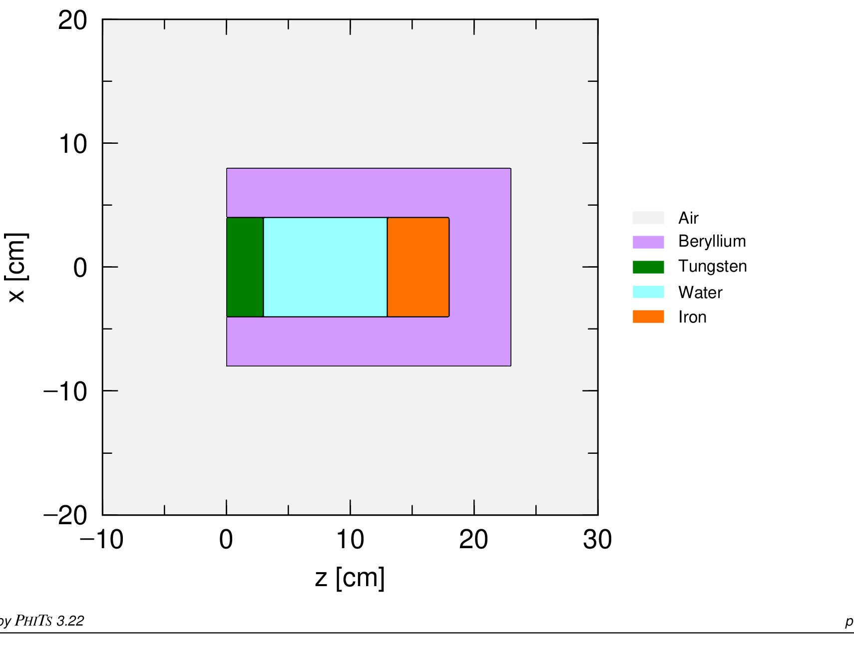
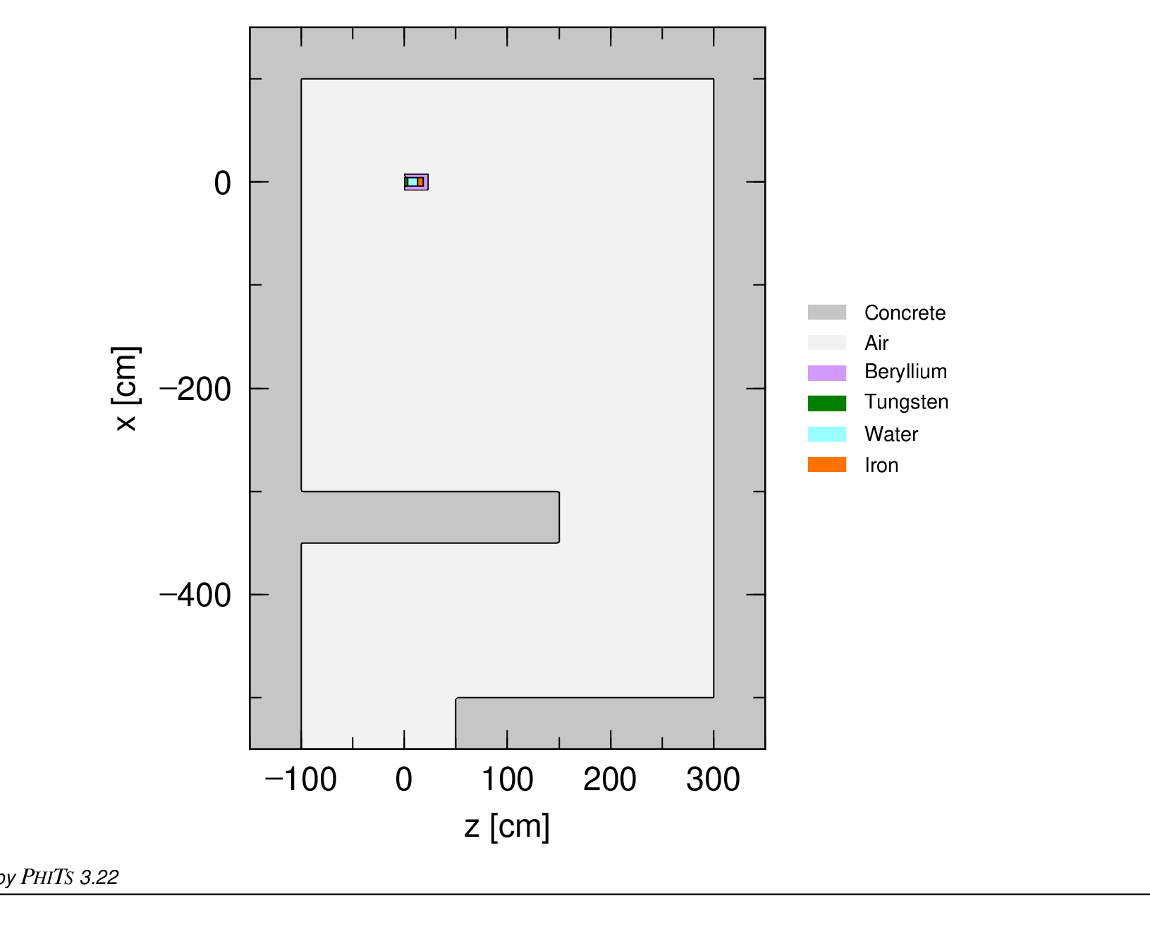
The PHITS input file used and modified throughout this example calculation can be found at <PHITS-install>/dchain-sp/sample/3-step_dose_xyz/phits_3-step.inp and is also shown in Appendix 6.3. It contains some commented lines and disabled sections which will be enabled later in the example. Most notably, this is the lines above the [Source] section for inserting a file, the room’s air and concrete regions in the [Cell] section, and the last [T-Track] tally. The two [G-Show] tallies were used to produce the images in Figures 4.13.1–4.13.2, and all output presented in this example will be produced automatically by PHITS or DCHAIN. Additionally, this example seeks to illustrate usage of xyz meshes with [T-Dchain] and how it can have notable impact on results in comparison to just reg meshes, depending on the scenario.

$ Photon source from DCHAIN output
$ infl:{W_reg_target_gamma_t3.pht}
$ This needs to come before the "off" source section or it will be skipped.

[Source]
   s-type =   1             # mono-energetic axial source
     proj =  proton         # kind of incident particle

\(\vdots\)

$ Room (void)
10  0          -16:(5 -20 15)   $ room + doorway air
11  0          -15:(20 -21 #10) $ outer + maze concrete walls
$ Room (with materials)
$ 10 10 -0.0012  -16:(5 -20 15)   $ room + doorway air
$ 11 11 -2.3     -15:(20 -21 #10) $ outer + maze concrete walls

\(\vdots\)

[T-Track] off
  title = Ambient dose equivalent H*(10) [mSv/hr] room map

For the sake of minimizing run time, the air and concrete cells (10 and 11) are filled with void instead of their respective materials for now; though it should be noted that the room geometry would have an impact on the neutron flux within the regions. Additionally, in a serious evaluation, one would want to simulate many more histories than 10,000 (maxcas\(\times\)maxbch=10,000 here), but is reduced here for speed. There are a number of other time-saving measures implemented in this example that will be pointed out.

Importantly, the [Parameters] required for [T-Dchain]/DCHAIN to function properly have been set, and the [Volume] for the regions of interest have been calculated. As a reminder, the [Volume] section is only necessary with reg meshes in [T-Dchain]; volumes are automatically calculated for xyz meshes. Variables have been declared to allow input of the beam current in nA which is then automatically converted to particles/sec for the [T-Dchain] amp parameter. There are three [T-Dchain] tallies. The first two are tallying over the same region, the tungsten target, but using differing meshes (reg and xyz), and the third [T-Dchain] tally is an xyz mesh covering the entire target block. The first [T-Track] tally is just a flux tally for particle fluxes in the target. After running this file in PHITS, this [T-Track] tally produces the plots shown in Figures 4.13.3–4.13.4.

$  required options for DCHAIN
 file(21) = c:/phits/dchain-sp/data # (D=c:/phits/dchain-sp/data) DCHAIN data folder
 jmout    =           1     # (D=0) Density echo, 0:input, 1:number density
 e-mode   =           0     # (D=0) Event generator mode is not recommended for DCHAIN
 igamma   =           3     # (D=2) 0:No, 1:Old, 2:EBITEM, 3:EBITEM+Isomer

\(\vdots\)

[Volume]   $ required section for DCHAIN
   reg   vol
     1   c1*(2*c5)**2
     2   c2*(2*c5)**2
     3   c3*(2*c5)**2
     4   ((c1+c2+c3+c4)*(2*c6)**2)-((c1+c2+c3)*(2*c5)**2)

Fig. 4.13.3 Proton flux

Fig. 4.13.4 Neutron flux

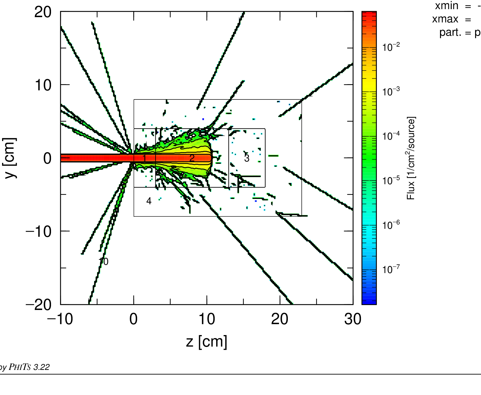
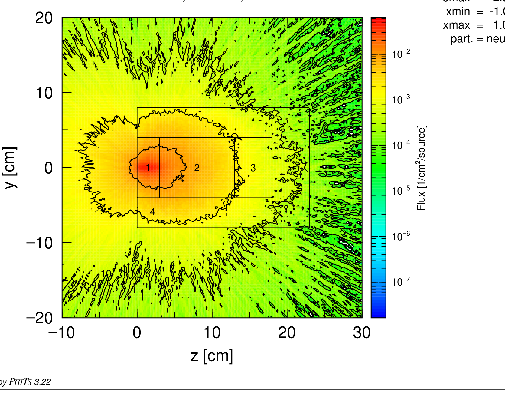
Additionally, three sets of DCHAIN input files have been generated, adopting the filenames provided to the file parameter in the [T-Dchain] tallies. Note that due to the temporary files generated by DCHAIN, only one DCHAIN simulation can be ran at a time in a single folder/directory, so they must either be ran sequentially or separated into separate folders to be ran simultaneously. For simplicity they will be ran sequentially here. In this example, DCHAIN is being controlled entirely through parameters provided to the [T-Dchain] tally (some of which are just passed along from PHITS to DCHAIN).

[T-DCHAIN]
  title = W target (reg)
  mesh = reg
  reg = 1
  file = W_reg_target.out     # file name of dchain input file
  timeevo =    2             # time evolution / irradiation schedule
    10.0 m 1.0
    50.0 m 0.0
  outtime =    4             # output times
    10.0 m
    -1 m
    -5 m
    -50 m
  amp = c12                  # (D=1.0) Source Intensity(source/sec)
  idivs = 50                 # (D=50) number of calculation substebs used in irradiation
  iphtout = 2                # (D=1) 2 = separate [Source] output to files for each time

Looking at the first [T-Dchain] tally (above), the mesh, output filename, time schedule of the beam / active source, requested output times, and nominal beam intensity are provided as is done normally as a baseline. The only additional parameter specified is iphtout= 2 which corresponds to the DCHAIN input PHITSOUT; setting it to 2 causes the PHITS [Source] cards outputted by DCHAIN to be written to separate files for each output time. The convenience of this will become apparent later. Run W_reg_target.out through DCHAIN, which should only take a few seconds to complete, and the usual output files will be generated. However, as specified, the *.pht output has been split into four files corresponding to each of the requested output times.

[T-DCHAIN]
  title = W target (xyz)
  mesh = xyz
  x-type = 2
      nx = 8
    xmin = -c5
    xmax =  c5
  y-type = 2
      ny = 8
    ymin = -c5
    ymax =  c5
  z-type = 2
      nz = 3
    zmin = 0
    zmax = c1
  file = W_xyz_target.out     # file name of dchain input file
  timeevo =    2             # time evolution / irradiation schedule
    10.0 m 1.0
    50.0 m 0.0
  outtime =    4             # output times
    10.0 m
    -1 m
    -5 m
    -50 m
  amp = c12                  # (D=1.0) Source Intensity(source/sec)
  idivs = 4                  # (D=50) number of calculation substebs used in irradiation
  iphtout = 2                # (D=1) 2 = separate [Source] output to files for each time
  ipltmode = 1               # (D=0) enable DCHAIN 2D xy activity plot

The second [T-Dchain] tally (above) nominally contains the same information except the region mesh reg has been substituted for a three-dimensional grid mesh xyz. The tungsten portion of the target has dimensions 8 cm \(\times\) 8 cm \(\times\) 3 cm, and the xyz mesh is set to divide the region into an 8\(\times\)8\(\times\)3 grid of 1 cm\(^3\) voxels. In addition to iphtout= 2, two other extra parameters have also been set. The first is idivs= 4 which controls how many steps each irradiation time step is subdivided into for the DCHAIN calculation. It has a default value of 50 which is a conservative general recommendation, particularly for neutron activation scenarios as it allows for nuclides to more accurately “grow in,” but what value of this is necessary is quite dependent on the half-lives of any important nuclides and the sizes of the time steps inputted into timeevo. For a problem whose activation is primarily dependent on output from [T-Dchain]’s [T-Yield] tally for high-energy reactions, such as is the case in this example, many divisions is not necessary. It has been reduced here to only 4 to speed up the calculation. As covered in Section 4.8, DCHAIN’s run time scales strongly with the number of regions (192 here) and IDIVS.

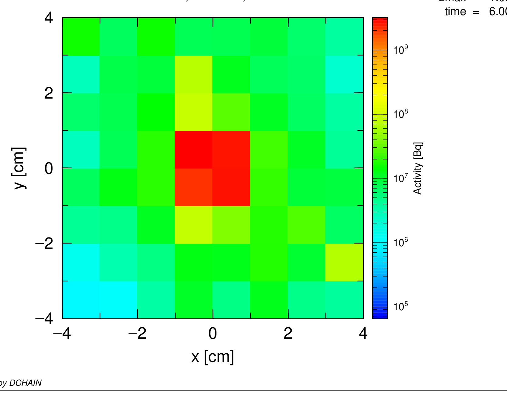
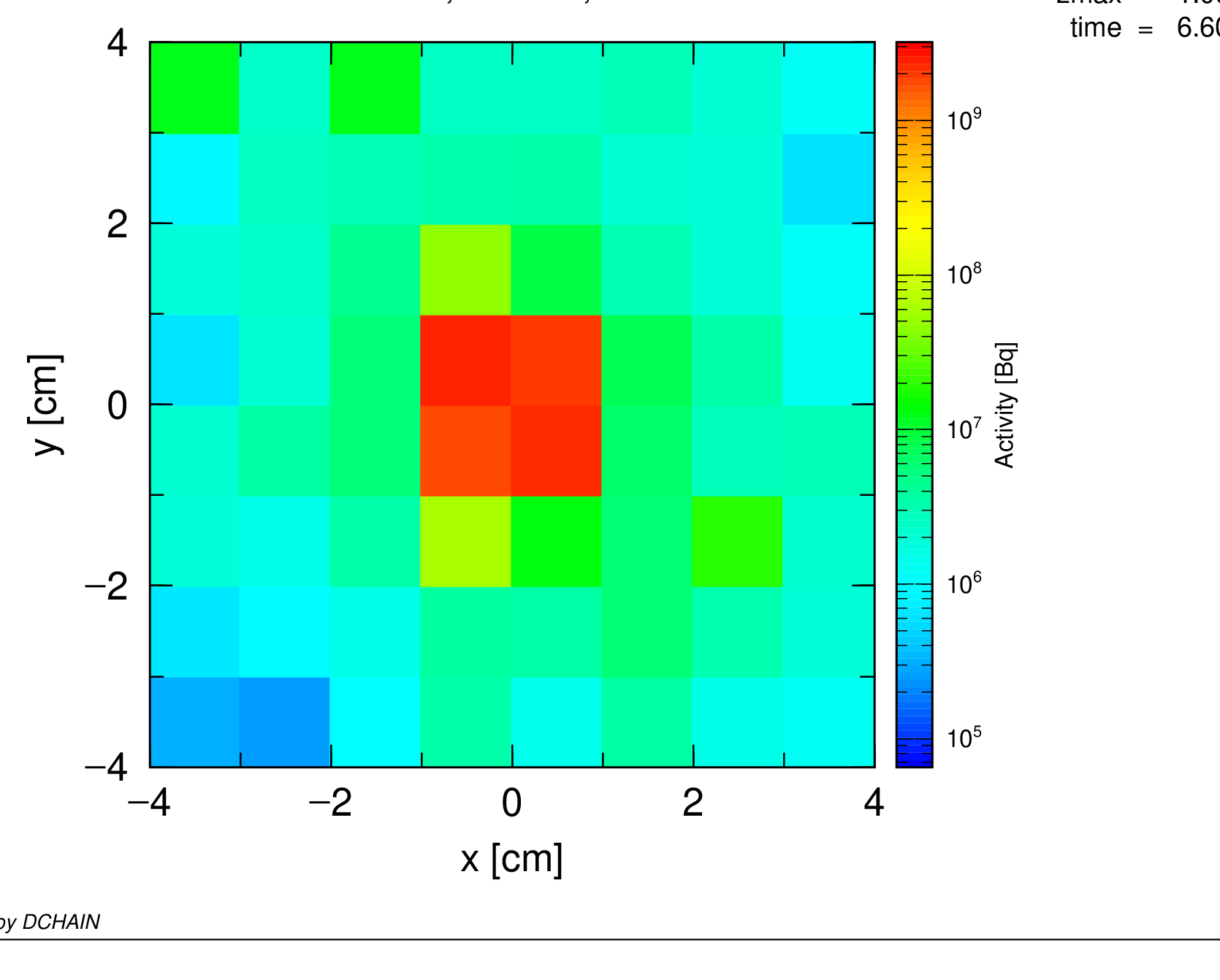
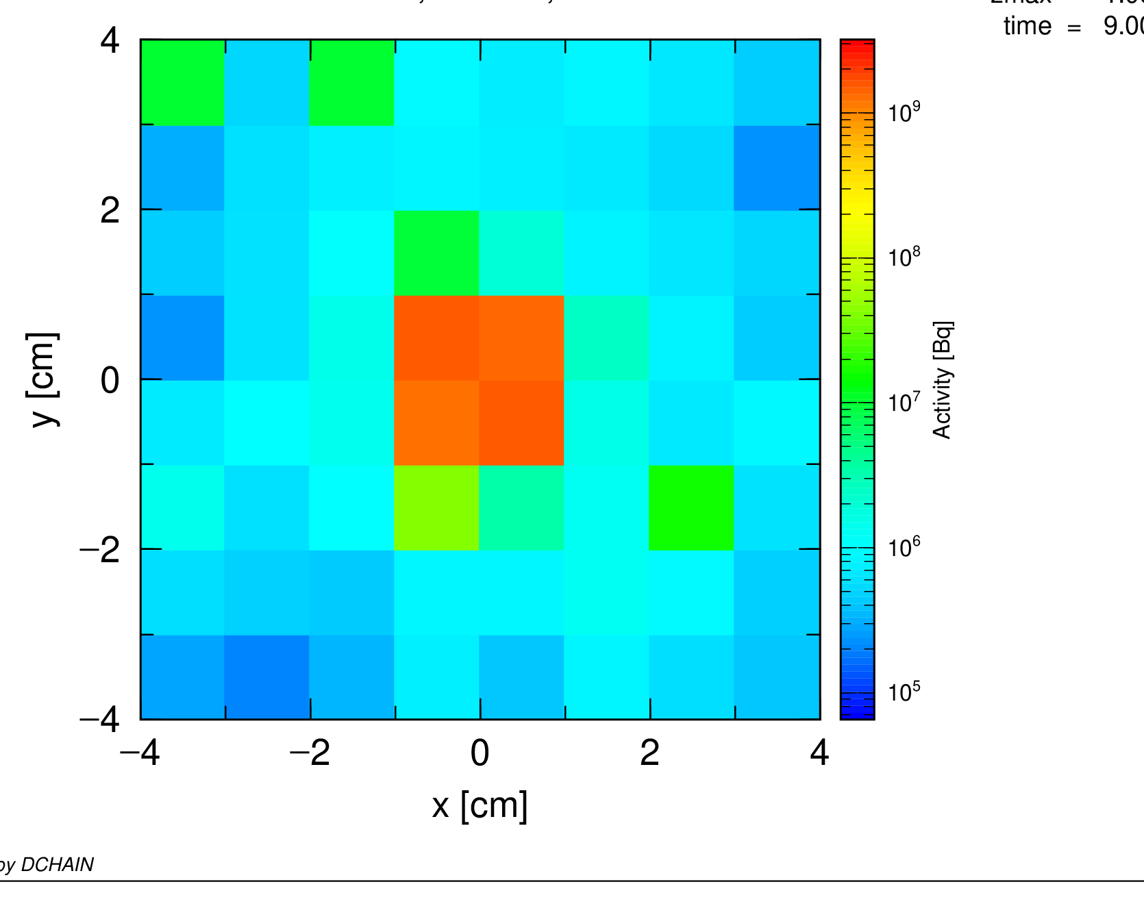
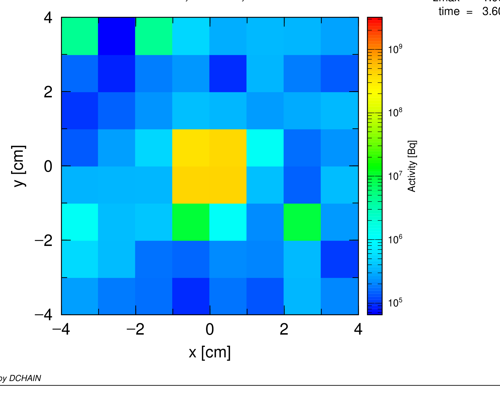
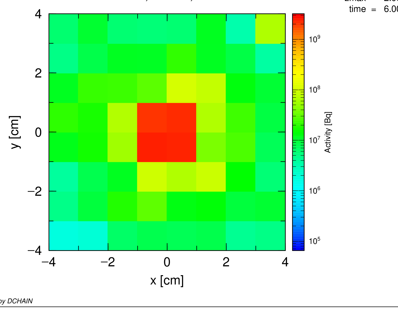
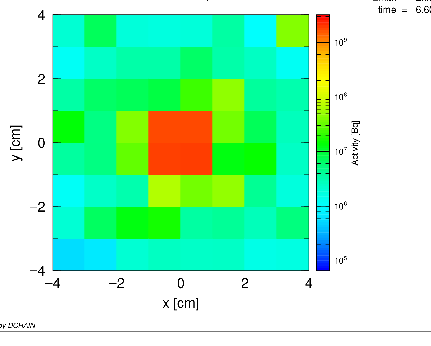
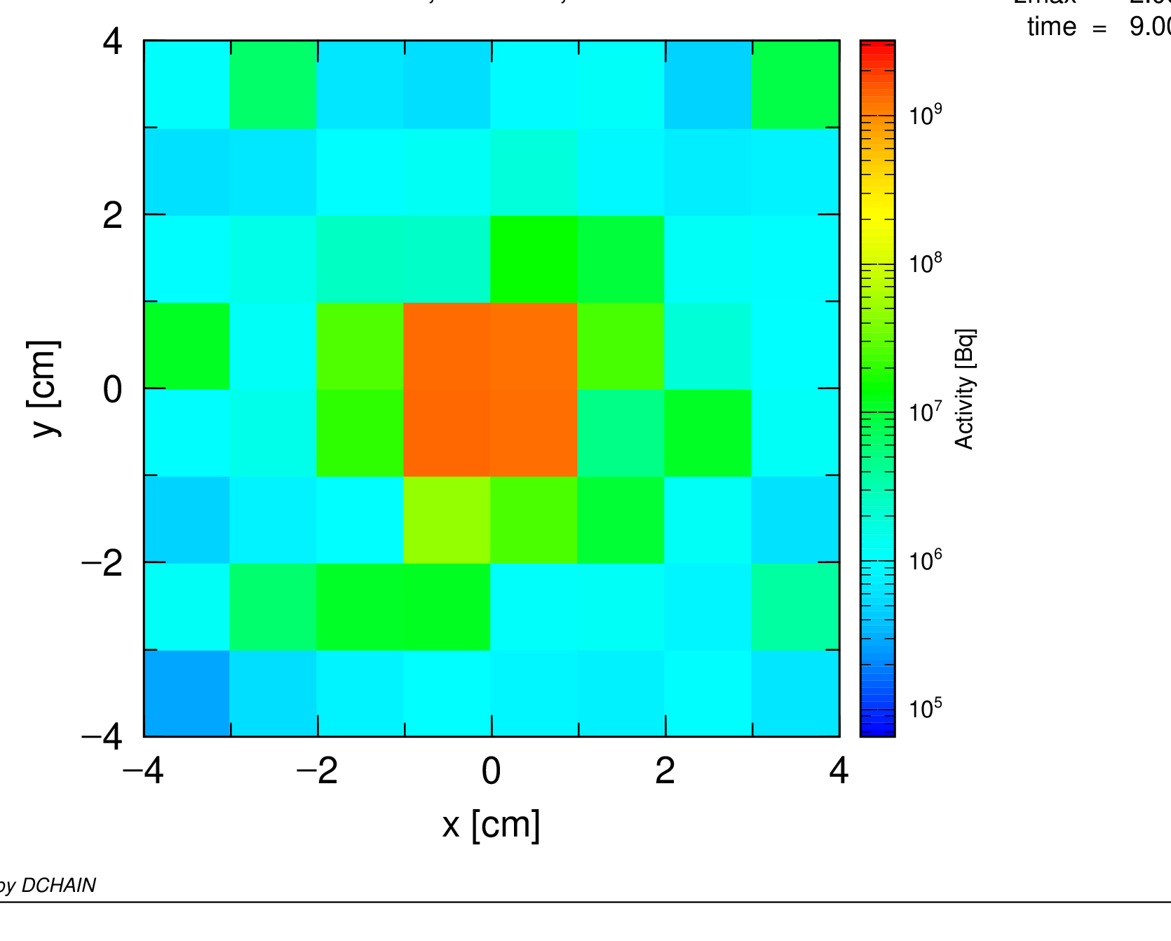
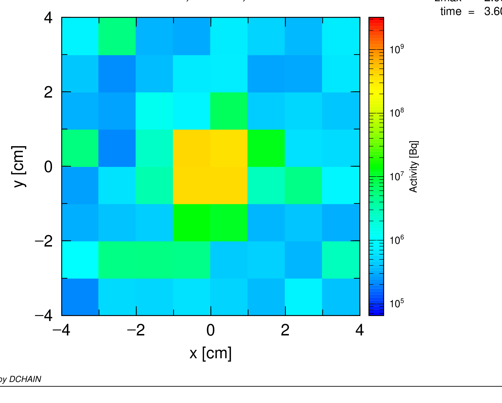
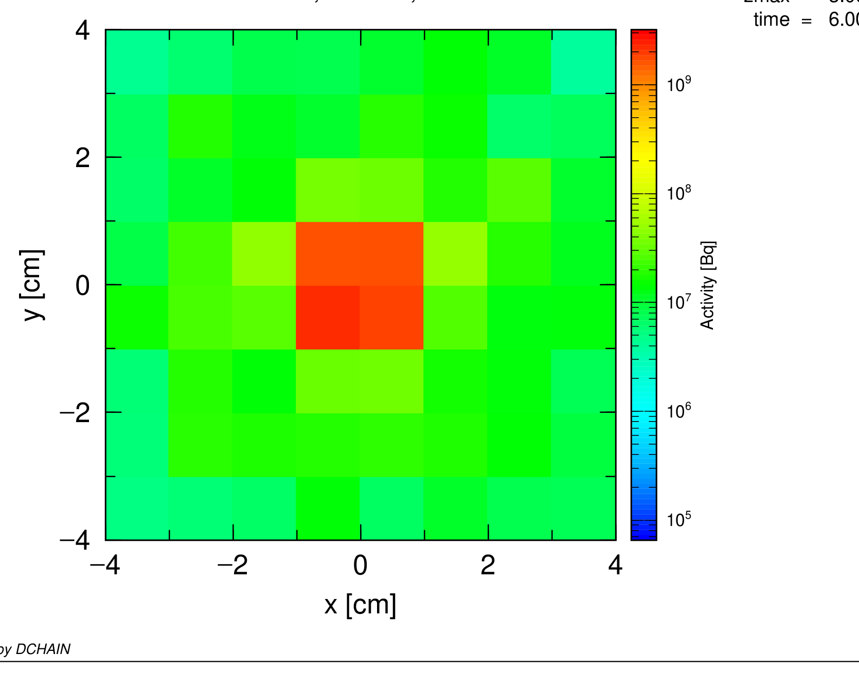
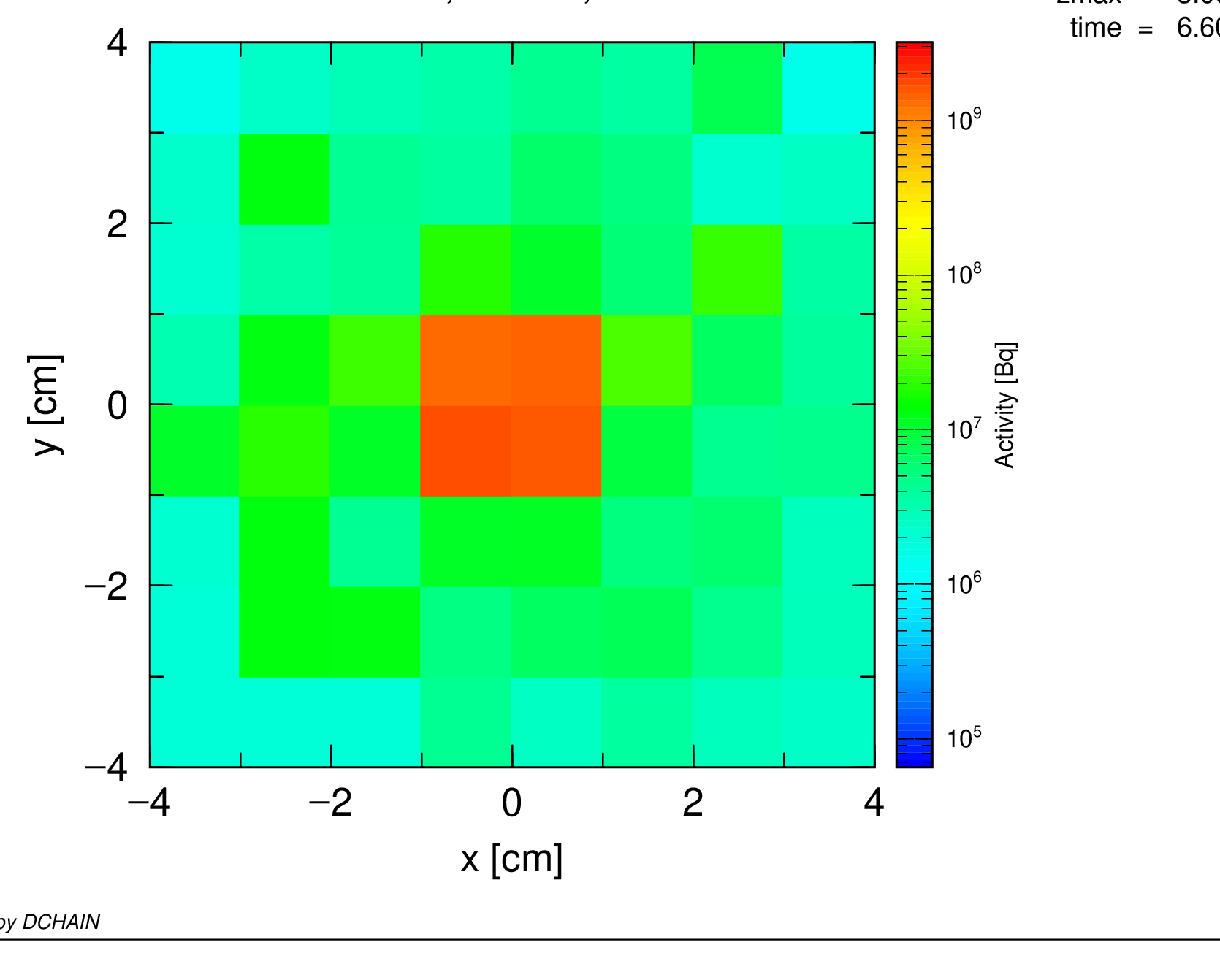
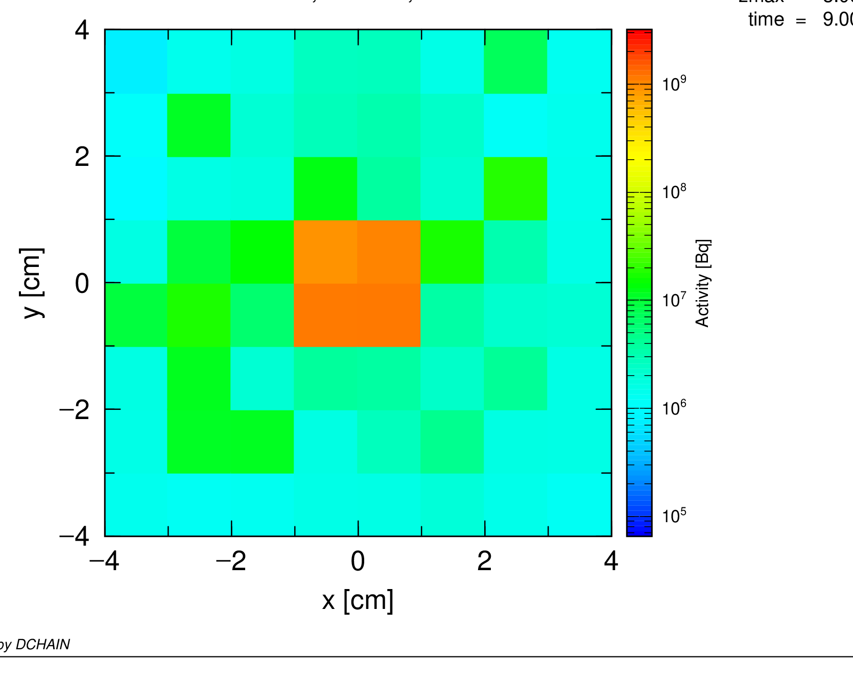
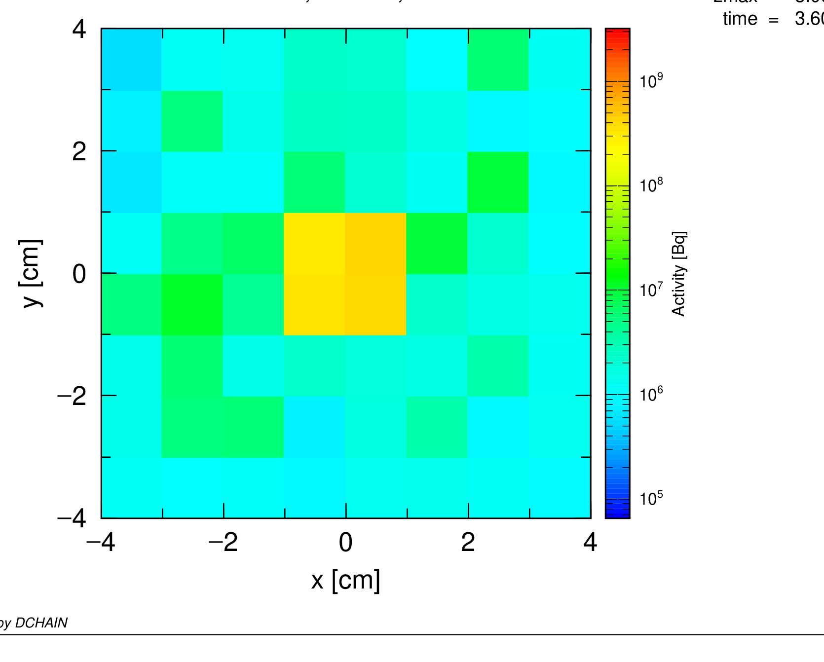
The other extra parameter provided to [T-Dchain] was ipltmode= 1 which tells DCHAIN to also output activity map plots sliced in the xy plane of the grid mesh. Run W_xyz_target.out through DCHAIN; despite reducing IDIVS, the much higher number of regions means this calculation will still take a bit longer than the previous one. In addition to the output files already discussed, W_xyz_target_pxy.eps (created from W_xyz_target_pxy.out) will also be produced. As set with ipltmode, this file shows plots of the mesh in the xy plane at each slice in z and at each output time. The results are shown in the activity plots below. As expected, activity is concentrated in the central region where the beam passed through, activity decreases with increasing cooling time, and the level of peripheral activation (outside of the beam trajectory) increases with depth in the target.

[T-DCHAIN]
  title = Whole target structure
  mesh = xyz
  x-type = 2
      nx = 1
    xmin = -c6
    xmax =  c6
  y-type = 2
      ny = 8
    ymin = -c6
    ymax =  c6
  z-type = 2
      nz = 12
    zmin = 0
    zmax = c1+c2+c3+c4
  file = whole_target_yz-view.out  # file name of dchain input file
  timeevo =    2             # time evolution / irradiation schedule
    10.0 m 1.0
    50.0 m 0.0
  outtime =    4             # output times
    10.0 m
    -10 s
     -1 m
    -50 m
  amp = c12                  # (D=1.0) Source Intensity(source/sec)
  idivs = 4                  # (D=50) number of calculation substebs used in irradiation
  ipltmode = 4               # enable DCHAIN 2D yz activity plot

The third [T-Dchain] tally (above) is structured very similarly to the second one. It has an xyz mesh encompassing the entire target block with dimensions 16 cm \(\times\) 16 cm \(\times\) 23 cm. Since a 1 cm resolution mesh would result in 5888 regions and take a substantially longer time to run in DCHAIN, some compromises are made. Since this tally’s purpose is primarily to show how activity changes with time in each region/material, the x direction is collapsed into a single bin, and the spatial resolution in the y and z directions is halved. Thus, the mesh used is 1 \(\times\) 8 \(\times\) 12 with each voxel having dimensions 16 cm \(\times\) 2 cm \(\times\) 1.9 cm for a total of only 96 voxels. The output times have also been slightly altered. Rather than being at 0, 1, 5, and 50 minutes after the end of irradiation, the output times for this plot are 0 sec, 10 sec, 1 min, and 50 min after the end of irradiation.

The idivs parameter is still set to 4, but the ipltmode parameter is now changed from 1 to 4, telling DCHAIN to output its two-dimensional activity plots in the yz plane, slicing along the x dimension (which has been reduced to a single bin in this case). Run whole_target_yz-view.out through DCHAIN, and a familiar set of outputs will be generated. However, note that this time there is only one *.pht file generated since the third [T-Dchain] tally did not alter iphtout from its default value of 1. These plots, contained in whole_target_yz-view_pyz.eps, are shown in Figures 4.13.5–4.13.8. From them we can see how activity diminishes rapidly from the Be region and more slowly in the W region. The notable fluctuations from voxel to voxel, in these and the previous plots, stem from the high variance coming from running the PHITS simulation for only 10,000 histories. Additionally, one should note that the number of histories needed for decent statistics in all of the voxels increases the finer the xyz mesh resolution is.

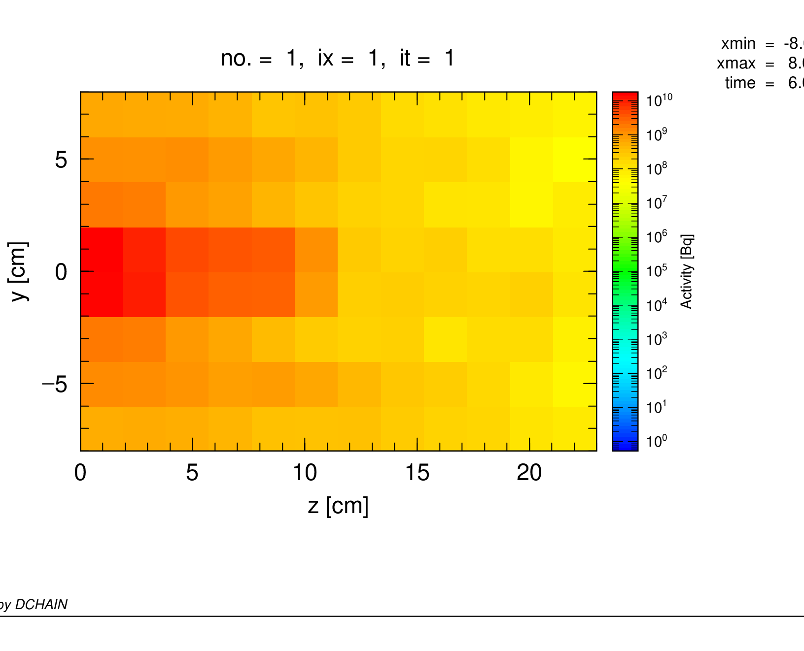
Fig. 4.13.5 t_cooling = 0 sec

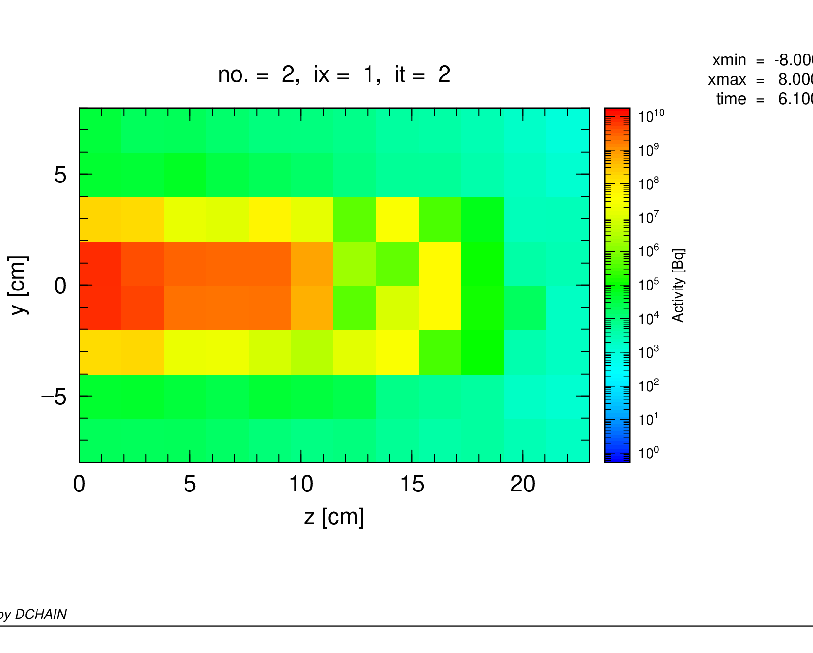
Fig. 4.13.6 t_cooling = 10 sec

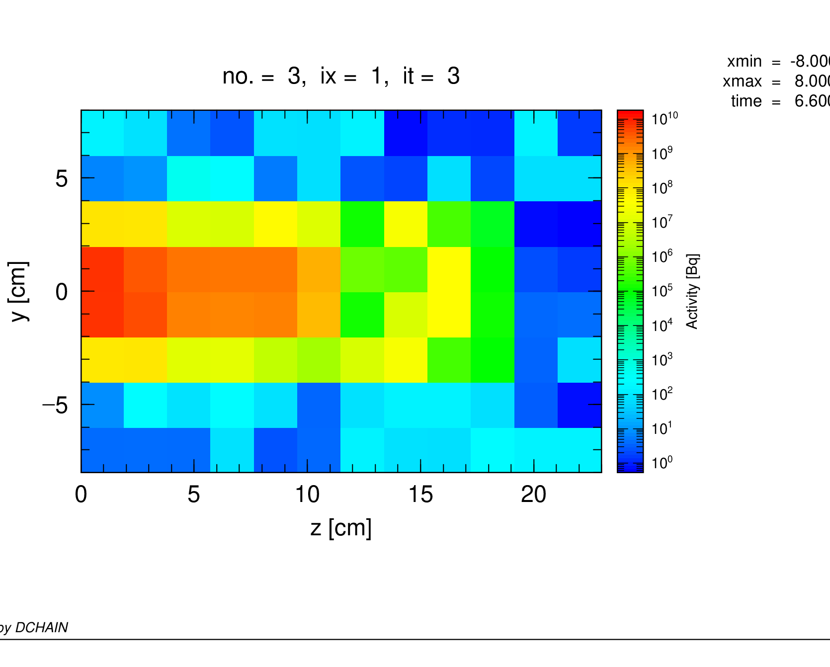
Fig. 4.13.7 t_cooling = 1 min

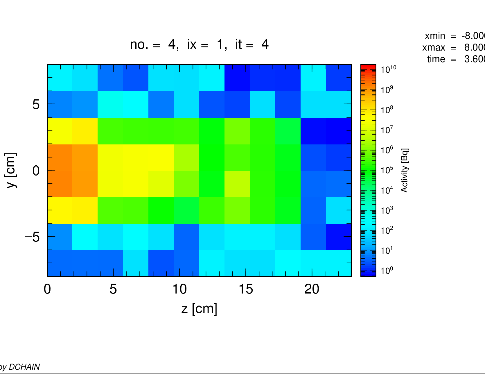
Fig. 4.13.8 t_cooling = 50 min

One note worth pointing out is that for the xyz mesh, an individual voxel within the mesh can contain multiple materials. The first xyz mesh was only over the tungsten portion of the target, but this one covered the entire target block with the boundaries of the grid not selected specifically to isolate individual materials to each voxel. This can be seen in the region definition portion of the DCHAIN input deck whole_target_yz-view.out; the first portion of which is shown below. Note that DCHAIN does not subdivide each voxel to keep the materials within them isolated; it just combines all of the materials within a voxel, treating it like a single region filled with a homogeneous mixture.

! --- calculation region details ---

      imat =      4
   mtscore =      0
   mt-list =      5
   W-180     7.5882E-05
   W-182     1.6756E-02
   W-183     9.0514E-03
   W-184     1.9376E-02
   W-186     1.7975E-02
   mt-list =      3
   H-1       6.6880E-02
   H-2       1.0033E-05
   O-16      3.3446E-02
   mt-list =      4
  Fe-54      4.9642E-03
  Fe-56      7.7928E-02
  Fe-57      1.7997E-03
  Fe-58      2.3951E-04
   mt-list =      1
  Be-9       1.2352E-01
     imesh =      96
   non    ix    iy    iz        fluxs       volume    volmat001    volmat002    volmat003    volmat004
     1     1     1     1   1.2681E+09   6.1333E+01   0.0000E+00   0.0000E+00   0.0000E+00   6.1333E+01
     2     1     2     1   2.8259E+09   6.1333E+01   0.0000E+00   0.0000E+00   0.0000E+00   6.1333E+01
     3     1     3     1   5.6903E+09   6.1333E+01   2.8395E+01   0.0000E+00   0.0000E+00   3.2938E+01
     4     1     4     1   1.7153E+10   6.1333E+01   2.8395E+01   0.0000E+00   0.0000E+00   3.2938E+01
     5     1     5     1   1.7210E+10   6.1333E+01   2.8395E+01   0.0000E+00   0.0000E+00   3.2938E+01
     6     1     6     1   5.6811E+09   6.1333E+01   2.8395E+01   0.0000E+00   0.0000E+00   3.2938E+01
     7     1     7     1   2.7261E+09   6.1333E+01   0.0000E+00   0.0000E+00   0.0000E+00   6.1333E+01
     8     1     8     1   1.2740E+09   6.1333E+01   0.0000E+00   0.0000E+00   0.0000E+00   6.1333E+01
     9     1     1     2   1.5936E+09   6.1333E+01   0.0000E+00   0.0000E+00   0.0000E+00   6.1333E+01
    10     1     2     2   3.7344E+09   6.1333E+01   0.0000E+00   0.0000E+00   0.0000E+00   6.1333E+01
    11     1     3     2   6.9048E+09   6.1333E+01   1.5863E+01   1.3542E+01   0.0000E+00   3.1929E+01
    12     1     4     2   1.5202E+10   6.1333E+01   1.5863E+01   1.3542E+01   0.0000E+00   3.1929E+01

Now that DCHAIN has been ran, the PHITS [Source] sections outputted by DCHAIN into the *.pht files can be reinserted into the PHITS input to simulate transport of the decay radiation. In this example, this process for both the reg and xyz meshes is demonstrated, and then the differences in the final results between the two will be compared. Before that, a few modifications will be made to the PHITS input.

Since we will be simulating decay-energy photons which are much faster to transport than 250 MeV protons and are not generating any activation we are interested in, let’s:

•\(\quad\) increase the number of particle histories per batch from 1000 to 100,000,

maxcas   =      100000     # (D=10) number of particles per one batch
maxbch   =          10     # (D=10) number of batches

•\(\quad\) disable the original source section,

[Source] off
   s-type =   1             # mono-energetic axial source
     proj =  proton         # kind of incident particle
       e0 =   250.00        # energy of beam [MeV/u]

•\(\quad\) replace the void in the room regions 10 and 11 with air and concrete,

$ Room (void)
$10  0          -16:(5 -20 15)   $ room + doorway air
$11  0          -15:(20 -21 #10) $ outer + maze concrete walls
$ Room (with materials)
10 10 -0.0012  -16:(5 -20 15)   $ room + doorway air
11 11 -2.3     -15:(20 -21 #10) $ outer + maze concrete walls

•\(\quad\) and disable the [T-Dchain] tallies.

[T-DCHAIN] off

\(\vdots\)

[T-DCHAIN] off

\(\vdots\)

[T-DCHAIN] off

Because surveying the differences in the photon flux profile within the target area will be interesting, let’s make the first [T-Track] tally only track photons and rename its output file to something we will be able to modify to make easily distinguishable between the reg and xyz [Source] sections from DCHAIN, in this case just adding “_reg-src” before the file extension. (We will look at the reg [Source] first.)

file = yz-track_reg-src.out
part = photon

Since we are interested in calculating the ambient dose equivalent rate distribution within the room, we will need to enable the second [T-Track] tally which has this calculation prepared.

$ Photon source from DCHAIN output
infl:{W_reg_target_gamma_t3.pht}
$ This needs to come before the "off" source section or it will be skipped.

[Source] off
   s-type =   1             # mono-energetic axial source
     proj =  proton         # kind of incident particle
       e0 =   250.00        # energy of beam [MeV/u]

There are a few things to note about this tally. From the y axis mesh and the geometry, we can see this tally is set up to tally the dose rate in the first two meters above the concrete floor coming from particles between 1 keV and 10 MeV. The factor is used to scale the output units from pSv/sec to mSv/hr, and the multiplier is set to multiply all fluxes in region 10 (the air) by \(H^*(10)\) fluence-to-dose conversion coefficients and to multiply fluxes in other regions by 0. The angel parameters are setting the bounds of the color bar that will appear in the output plot. Normally these are set well automatically, but since we will be comparing results from two different simulations (reg versus xyz) as the primary result, it is best to ensure their scales will be exactly identical. Also note that the name provided to file is formatted similarly to the one set for the other [T-Track] tally in regards to easily distinguishing between the reg and xyz mesh cases.

All that remains to address is the [Source] section containing the decay radiation spectrum being emitted from the tungsten portion of the target. Above the original [Source] is a line for inserting a file via the infl function. Uncommenting that line will cause the contents of W_reg_target_gamma_t3.pht to be inserted into the PHITS input.

[T-Track]
  title = Ambient dose equivalent H*(10) [mSv/hr] room map
  mesh = xyz
  x-type = 2
      nx =  140
    xmin = -550
    xmax =  150
  y-type = 2
      ny = 1
    ymin = -100
    ymax =  100
  z-type = 2
      nz =  100
    zmin = -150
    zmax =  350
    unit = 1
    axis = xz
  e-type = 3
      ne = 1
    emin = 0.001
    emax = 10
  file = room-dose_reg-src.out
  set:c20[3600/1.0E+09]
  factor = c20       $ convert pSv/sec to mSv/hr
  multiplier = 6     $ number of regions using multiplier
     mat    mset1
     1    ( 0 -200 ) $ Zero out regions where we don't
     2    ( 0 -200 ) $   care about the dose (inside walls
     3    ( 0 -200 ) $   and the target).
     4    ( 0 -200 )
     10   ( 1 -200 ) $ We only want to tally dose rate in air.
     11   ( 0 -200 )
  2D-type =  7   # 1:Cont, 2:Clust, 3:Color, 4:xyz, 5:mat, 6:Clust+Cont, 7:Col+Cont
  gshow =    1   # 0: no 1:bnd, 2:bnd+mat, 3:bnd+reg 4:bnd+lat
  epsout = 1         $ automatically generate eps plot
  $ Set bounds of ANGEL plot color bar and make axis labels bigger
  angel = cmin(1.0E-5) cmax(1.0E+1)
  sangel = 2
  x: {\Large z [cm]}
  y: {\Large x [cm]}

Recall that due to selecting iphtout= 2 in [T-Dchain] (PHITSOUT= 2 in DCHAIN), the decay radiation spectra for all regions is separated into individual files for each output time step. As the “t3” in the filename suggests, this file is for the third output time requested, 5 minutes after the end of the irradiation time step. Had iphtout been left at its default value of 1, we would also need to specify in the infl function the line numbers in the single *.pht file corresponding to the [Source] section for the third output time.

However, before we can run this, some modifications need to be made to the [Source] section in W_reg_target_gamma_t3.pht. The top portion of this file is shown below. The [Source] uses s-type = 5 (same as s-type = 2) wherein a region is selected and the user must construct a box around that region. PHITS will then, for every history, sample points randomly within this box until one is found which lies within the specified region. While the cell number provided to the reg = parameter here should be automatically entered correctly by DCHAIN, it cannot automatically construct this box since it is not spatially aware of cells in a reg mesh.

c <>-<>-<>-<>-<>-<>-<>-<>-<>-<>-<>-<>-<>-<>-<>-<>-<>-<>-<>
c <>-<>   no.     1  regionwise calculation data     <>-<>
c <>-<>   region label : DUMMY001                    <>-<>
c <>-<>-<>-<>-<>-<>-<>-<>-<>-<>-<>-<>-<>-<>-<>-<>-<>-<>-<>
c      no.  3   region=       1   output time=        15 [m]  (after the last shutdown=         5 [m])
c      --------------------------------------------------------------------------------
[ S o u r c e ]
 totfact =   2.9969E+10  $ total number of gamma-rays (n/sec/cc) x volume (cc)
  s-type =   5
    proj = photon
     reg =        1 $ This cell ID  should be revised for lattice  or combined cell case
      x0 =        $ Input minimum x of the region here
      x1 =        $ Input maximum x of the region here
      y0 =        $ Input minimum y of the region here
      y1 =        $ Input maximum y of the region here
      z0 =        $ Input minimum z of the region here
      z1 =        $ Input maximum z of the region here
     dir = all
  e-type = 4
      ne =     28
$     Energy  Flux (arbitrary unit)
$             ^^^^ Energy spectra (n/sec/cc) based on activity concentration (Bq/cc)
      0.0010  1.4968E+06
      0.0100  2.2244E+05
      0.0200  3.3342E+06
      0.0300  3.7151E+06

Thus, we must add the boundaries of this box to the [Soruce] section manually. To maximize efficiency, it is best to make the box constrain the region fairly tightly (but still contain all of the region). Since in this case the specified region is actually in the shape of a box, we can provide it with the exact dimensions as shown below.

reg =        1 $ This cell ID  should be revised for lattice  or combined cell case
 x0 =  -4    $ Input minimum x of the region here
 x1 =   4    $ Input maximum x of the region here
 y0 =  -4    $ Input minimum y of the region here
 y1 =   4    $ Input maximum y of the region here
 z0 =   0    $ Input minimum z of the region here
 z1 =   3    $ Input maximum z of the region here

One more thing to note is that the value assigned to totfact will scale the PHITS results to the actual decay emission intensity. In this case, the whole tungsten region is emitting 2.9969E+10 photons per second. This value is calculated by just multiplying the total volumetric gamma flux, 1.5609E+08 here (written to the *.act file, as shown below), by the volume of the region: 8 cm \(\times\) 8 cm \(\times\) 3 cm = 192 cm\(^3\). And 1.5609E+08 \(\gamma\)/(cm\(^3\cdot\)sec) \(\times\) 192 cm\(^3\) = 2.9969E+10 \(\gamma\)/sec.

total gamma-ray flux                  1.5609E+08 +/- 7.5486E+06 (  4.84%) [n/s/cc]

A brief aside to explain the units conversions involved in the \(\dot{H}^*(10)\) [T-Track] tally is now warranted. The basic units of the [T-Track] tally with unit = 1 are \(\#\)/cm\(^2\) per source particle. Due to this totfact set in the [Source], the results are scaled by the emission rate whose units are \(\gamma\)/sec. Additionally, the fluence-to-dose conversion coefficients used by the multiplier section in the [T-Track] tally have units of pSv\(\cdot\)cm\(^2\)/particle (\(\gamma\) here). And lastly, the tally’s factor is set to change these units of time from seconds to hours and units of dose from pSv to mSv. Thus, these are all combined as shown below to obtain the tally’s final output units of mSv/hr.

\[\begin{equation*} \frac{\#}{\text{cm}^2} \cdot \frac{\gamma}{\text{sec}} \cdot \frac{\text{pSv}\cdot\text{cm}^2}{\gamma} \cdot \frac{\text{mSv}/\text{pSv}}{\text{hr}/\text{sec}} = \frac{\text{mSv}}{\text{hr}} \end{equation*}\]

Now that the [Source] section is prepared, now we can run the dchain_ex-dose.inp PHITS input file through PHITS again. This will generate the files specified in the two [T-Track] tallies which are shown in Figures 4.13.9–4.13.10. Note that while the units printed to the color bars read “Flux [1/cm\(^2\)/source]” the actual units are as previously discussed. In Figure 4.13.9, the photon flux has units of \(\gamma\)/(cm\(^2\cdot\)sec), and in Figure 4.13.10 the ambient dose equivalent rate has units of mSv/hr. These plots can be modified by changing labels, sizes, etc. in the *.out file and running it through ANGEL; the specification of this colorbar’s label is located near the very bottom of these files.

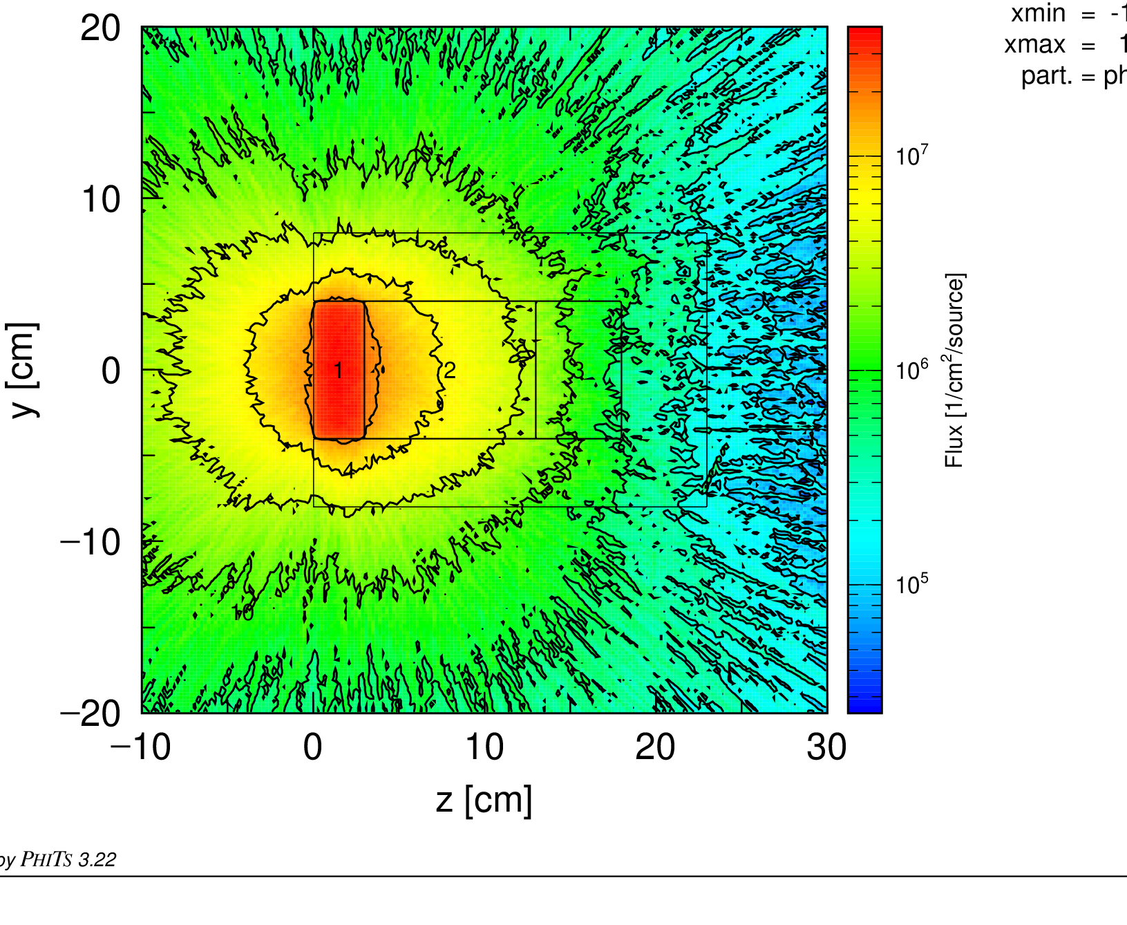
Fig. 4.13.9 Activated tungsten decay photon flux [\(\frac{\gamma}{\text{cm}^2\cdot\text{sec}}\)] in the target block

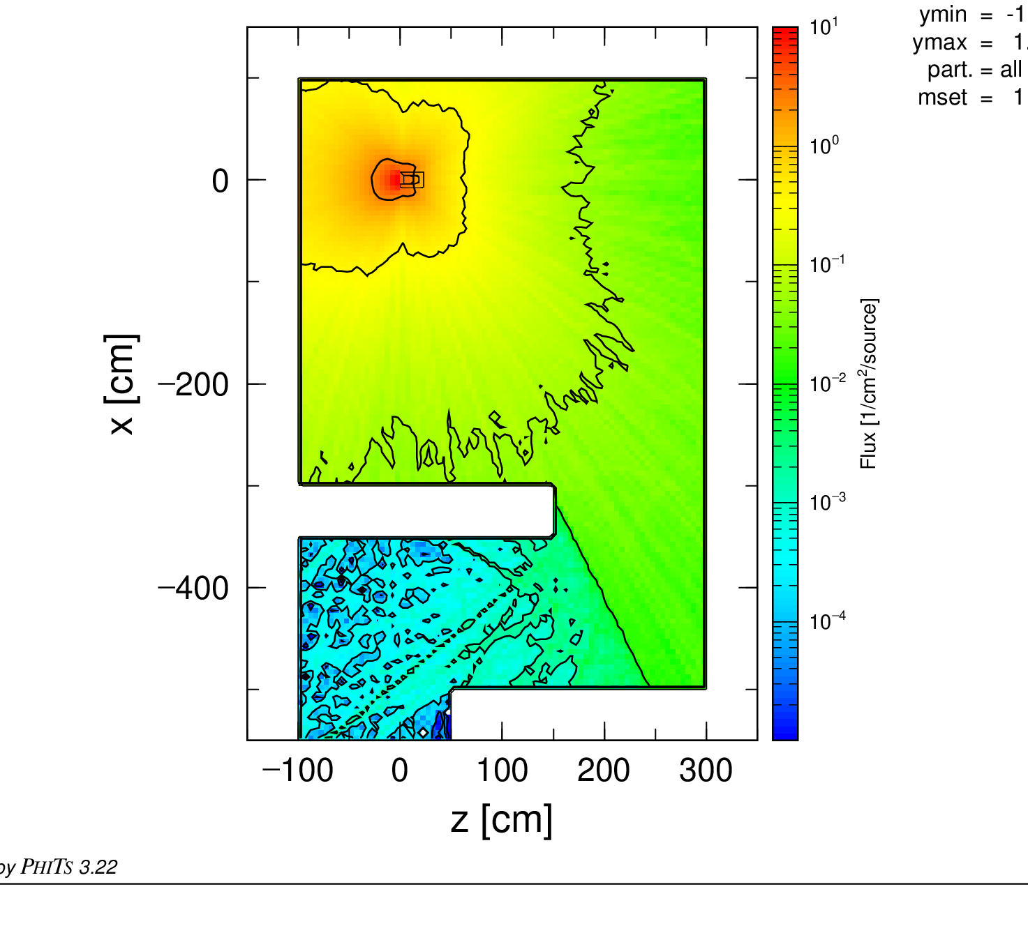
Fig. 4.13.10 \(\dot{H}^*(10)\) [mSv/hr] room map

For comparison, let’s repeat this for the mesh = xyz case. We need to make only a few modifications to the PHITS input file:

•\(\quad\) change the filename provided to the infl function to the *.pht file corresponding to the xyz mesh run at the same output time

$ Photon source from DCHAIN output
infl:{W_xyz_target_gamma_t3.pht}
$ This needs to come before the "off" source section or it will be skipped.

•\(\quad\) and change the output file names in the two [T-Track] tallies to now reflect our usage of the xyz mesh instead of the reg mesh.

file = yz-track_xyz-src.out

file = room-dose_xyz-src.out

And that’s it! Unlike with the reg mesh, the *.pht files produced for xyz meshes by DCHAIN have the source box dimensions already specified since the mesh’s grid structure is included in the PHITS tally output and passed to DCHAIN. Still, it is instructive to take a closer look at how the *.pht files produced for xyz meshes differ from those for reg meshes; a portion of the first section of W_xyz_target_gamma_t3.pht is shown below.

c <>-<>-<>-<>-<>-<>-<>-<>-<>-<>-<>-<>-<>-<>-<>-<>-<>-<>-<>
c <>-<>   no.     1  regionwise calculation data     <>-<>
c <>-<>   region label : xyz.000001                  <>-<>
c <>-<>-<>-<>-<>-<>-<>-<>-<>-<>-<>-<>-<>-<>-<>-<>-<>-<>-<>
c      no.  3   region=       1   output time=        15 [m]  (after the last shutdown=         5 [m])
c      ---------------------------------------------------------------------------------
 [ S o u r c e ]
<Source> =   2.8071E+05  $ total number of gamma-rays (n/sec/cc) x volume (cc) in this xyz voxel at this time
 totfact =   2.8071E+05  $ total number of gamma-rays (n/sec/cc) x volume (cc) summed over all preceeding regions at this time; only totfact from final <source> will be used
  s-type =   5
    proj = photon
     reg = all  $ This cell ID should be revised for lattice or combined cell case
      x0 = -4.000000E+00 $ Minimum x of the region
      x1 = -3.000000E+00 $ Maximum x of the region
      y0 = -4.000000E+00 $ Minimum y of the region
      y1 = -3.000000E+00 $ Maximum y of the region
      z0 =  0.000000E+00 $ Minimum z of the region
      z1 =  1.000000E+00 $ Maximum z of the region
     dir = all
  e-type = 4
      ne =     25
$     Energy  Flux (arbitrary unit)
$             ^^^^ Energy spectra (n/sec/cc) based on activity concentration (Bq/cc)
      0.0010  1.2268E+01
      0.0100  2.6172E+01
      0.0200  3.0745E+01
      0.0300  3.5958E+01
      0.0450  5.2974E-03
      0.0600  5.1652E+02
      0.0700  3.4553E+04

First, note that reg = all is used rather than providing reg = with a specific cell number; this is done for xyz meshes because a single voxel may contain portions of multiple cells. And perhaps the most obvious differences are the presence of <Source> = 2.8071E+05 and that the file is much longer now, containing <Source> sections for every voxel of the xyz mesh’s grid. This is the syntax for the multi-source in PHITS which allows simultaneous use of multiple source sections. The values of the <Source> entries just tell PHITS what the intensity of each <Source> section is relative to the others, and these <Source> values are normalized to unity upon being read into PHITS. The actual scaling of the output is controlled by the totfact parameter. While you may notice that every <Source> section has been provided with a totfact value, PHITS in fact will only use the final totfact value provided in a given [Source] section. The totfact values listed in each region is a running sum of the total emission rate for that and all preceding voxels. The top portion of the <Source> entry for the final voxel is shown below.

c <>-<>   no.   192  regionwise calculation data     <>-<>
c <>-<>   region label : xyz.000192                  <>-<>
c <>-<>-<>-<>-<>-<>-<>-<>-<>-<>-<>-<>-<>-<>-<>-<>-<>-<>-<>
c      no.  3   region=     192   output time=        15 [m]  (after the last shutdown=         5 [m])
c      ---------------------------------------------------------------------------------
<Source> =   1.3708E+06  $ total number of gamma-rays (n/sec/cc) x volume (cc) in this xyz voxel at this time
 totfact =   2.9969E+10  $ total number of gamma-rays (n/sec/cc) x volume (cc) summed over all preceeding regions at this time; only totfact from final <source> will be used
  s-type =   5
    proj = photon
     reg = all  $ This cell ID should be revised for lattice or combined cell case
      x0 =  3.000000E+00 $ Minimum x of the region
      x1 =  4.000000E+00 $ Maximum x of the region
      y0 =  3.000000E+00 $ Minimum y of the region
      y1 =  4.000000E+00 $ Maximum y of the region
      z0 =  2.000000E+00 $ Minimum z of the region
      z1 =  3.000000E+00 $ Maximum z of the region
     dir = all

Note that for this final voxel the totfact value, 2.9969E+10, is equal to the same total photon emission rate as was in the reg mesh [Source] section, as it should be. Since it is the final totfact value listed in this [Source] section, it is the one which will be applied to scale all results. We can run the updated dchain_ex-dose.inp input file through PHITS one last time, and the value of totfact used by PHITS can be verified from the input echo section of the phits.out file, shown below.

[ Source ]
  totfact =  2.99690E+10    # (D=1.0) global factor

The sign of totfact in a multi-source controls how the individual <Source> sections are sampled. When totfact is positive, all source particles will be born with the same weight, and the rate at which each <Source> section is sampled scales with its value relative to the values of other <Source> sections. (<Source> sections with higher values are sampled more often.) When totfact is negative, all <Source> sections are sampled equally but the weights of the particles spawned by each <Source> section are adjusted to reflect the relative intensity of that <Source> section against the other <Source> sections. By default it is positive, but if you wish to change this since the activities in an xyz mesh can often vary multiple orders of magnitude and you may wish to ensure that every single voxel is sufficiently sampled, only the final totfact value needs to be made negative.

It should also be noted that setting iphtout= 2 in [T-Dchain] (PHITSOUT= 2 in DCHAIN) is essentially mandatory for xyz meshes if you have more than one output time requested in outtime in [T-Dchain] (ITOUT in DCHAIN). This is because DCHAIN performs its calculations for one region at a time, meaning normally output for all time steps is written for a region before advancing to the next region. This is how the *.act file is structured and how the *.pht files are structured by default, if not split apart as done here. However, for this type of simulation, we want to isolate the decay spectra for all regions at a single time rather than for a single region at all times. If we had used iphtout= 1 here, we would have to tediously provide the infl function in PHITS with 192 different sets of line ranges containing all of the different <Source> sections at our single desired time or just only include the single output time in outtime.

Anyways, now that PHITS has been ran with the xyz mesh multi-source, we can observe its outputs, shown in Figures 4.13.11–4.13.12.

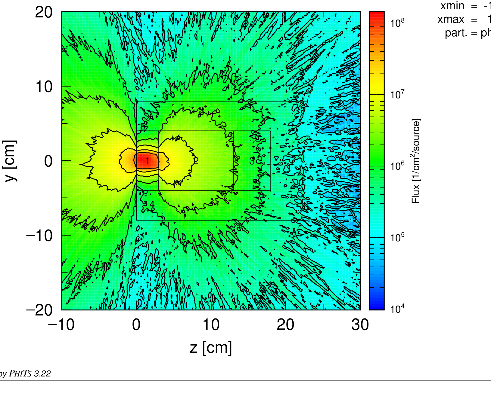
Fig. 4.13.11 Activated tungsten decay photon flux [\(\frac{\gamma}{\text{cm}^2\cdot\text{sec}}\)] in the target block

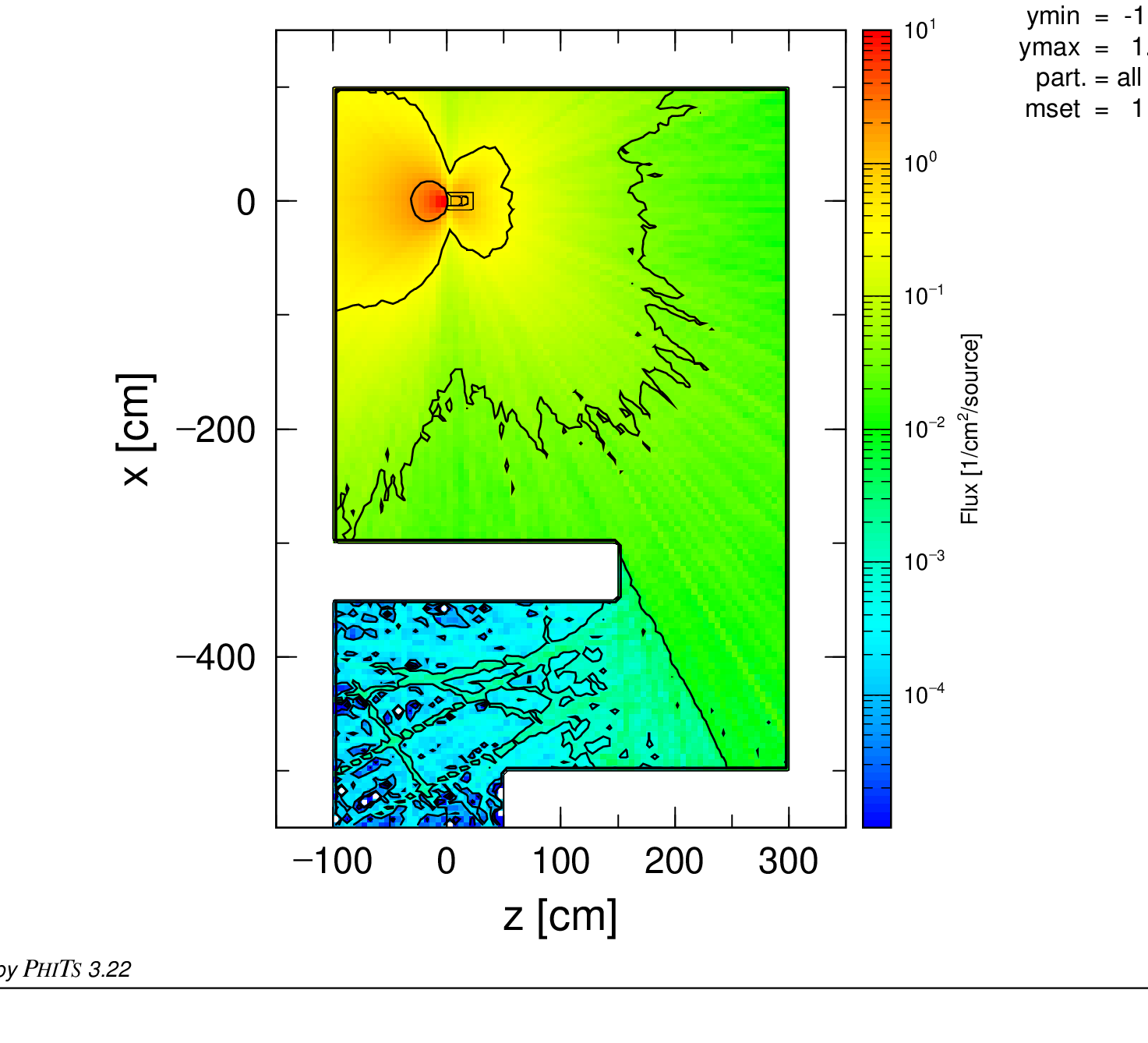
Fig. 4.13.12 \(\dot{H}^*(10)\) [mSv/hr] room map

For the reg mesh, the activation and resulting decay emissions were evenly distributed throughout the entire tungsten region. However, now with the xyz mesh, we can see that the emissions are indeed more narrowly concentrated along the path of the beam as had already been witnessed in the 2D xyz activity map plots produced by DCHAIN. This results in a noticeable self-shielding effect as a large fraction of photons are born toward the center (further from the exterior) of the tungsten target and are attenuated before escaping the target block. This has the ultimate effect of reducing the ambient dose equivalent rate in the room due to a greater fraction of emissions not escaping the target. One may note that the statistical clarity of these results seems slightly worse than those for the reg mesh despite the same number of original beam proton and decay photon histories being simulated in each case, and this is the reason. The same number of source photons are produced in both simulations, but for the xyz mesh case more are born toward the center of the target and are attenuated before escaping into the room.

Of course, statistics can always be improved by just running PHITS for more particle histories. Figures 4.13.13–4.13.16 show how these plots, for both reg and xyz cases, change when increasing the number of histories from 1 million to 50 million, making the effects of self-shielding on the photon flux around the target and resulting reduction in \(\dot{H}^*(10)\) in the room more apparent. (The colorbar labels have been adjusted in ANGEL too.)

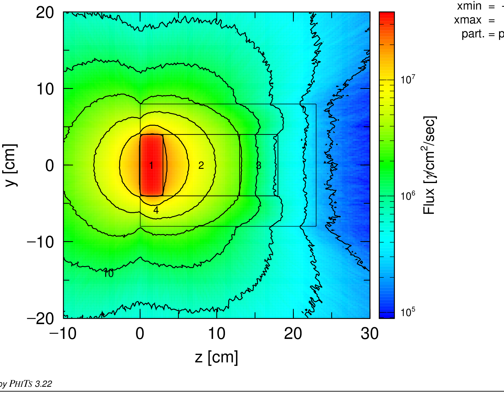
Fig. 4.13.13 reg - Activated tungsten decay photon flux [\(\frac{\gamma}{\text{cm}^2\cdot\text{sec}}\)] in the target block

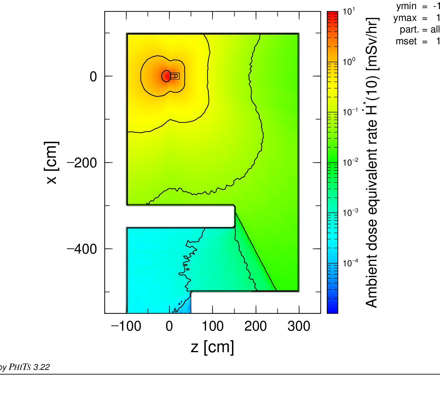
Fig. 4.13.14 reg - \(\dot{H}^*(10)\) [mSv/hr] room map

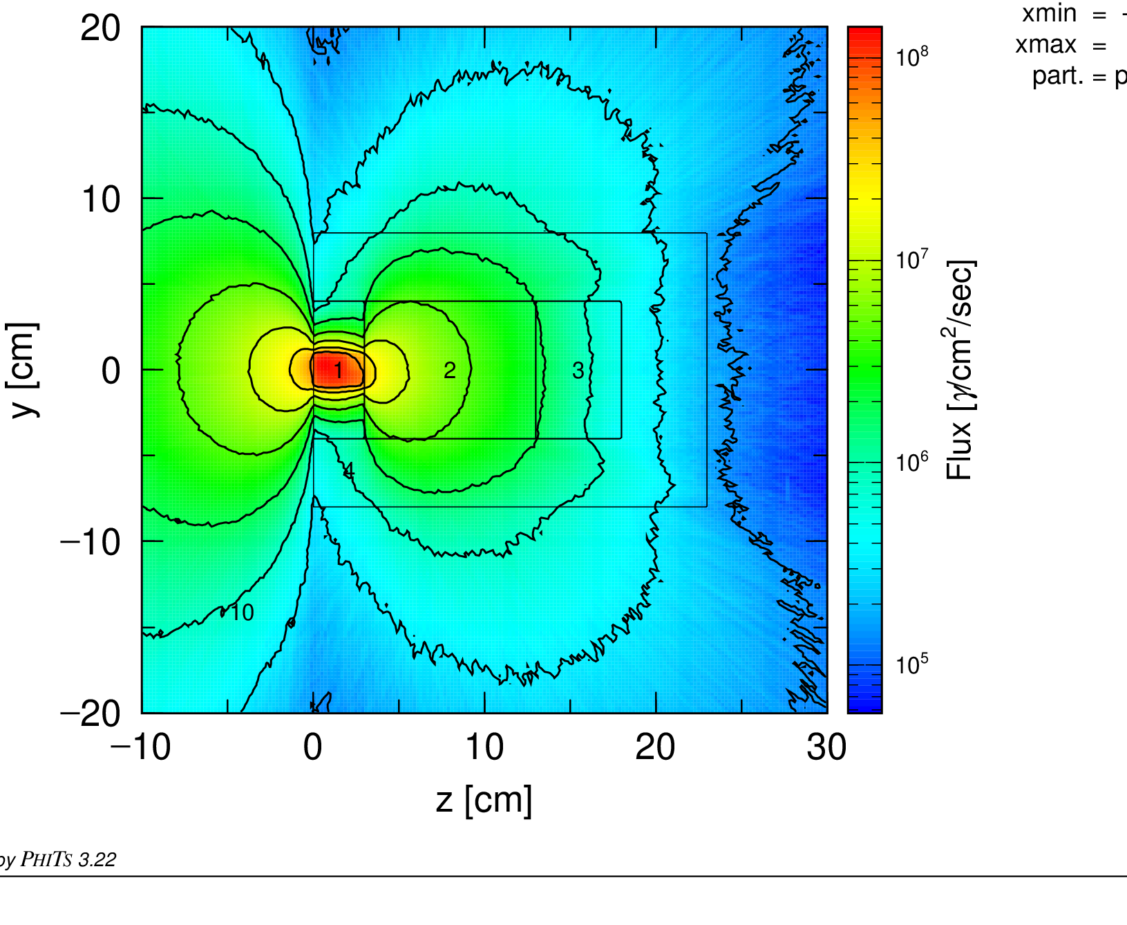
Fig. 4.13.15 xyz - Activated tungsten decay photon flux [\(\frac{\gamma}{\text{cm}^2\cdot\text{sec}}\)] in the target block

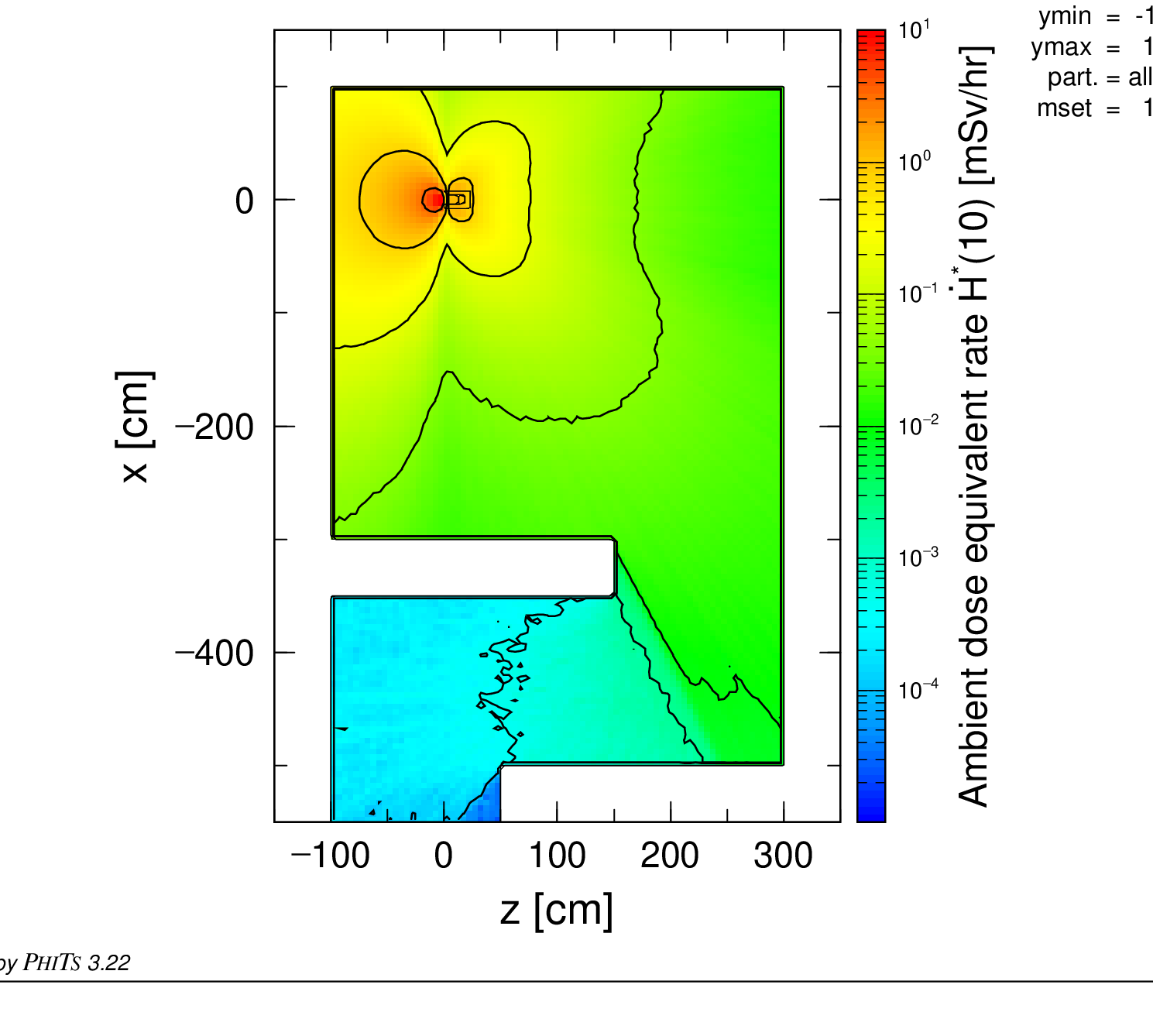
Fig. 4.13.16 xyz - \(\dot{H}^*(10)\) [mSv/hr] room map

For the sake of illustration, Figures 4.13.17–4.13.18 show how the xyz plots, still with 50 million histories, would change if the totfact value had been made negative instead (by changing the sign of the final totfact in W_xyz_target_gamma_t3.pht). Perhaps counterintuitively, the statistical clarity actually gets worse despite the voxels nearest the edge of the target being sampled more. Studying the *.gso and *.act files, one will see that the photons contributing the most to dose rate and with the most penetrating power are ones from nuclides created through high-energy beam reactions in the tungsten, and in the xyz mesh case they are only being spawned a significant fraction of the time in the voxels closest to the center of the target. Additionally, due to setting totfact as a negative value in order to sufficiently sample all voxels, it does mean that these voxels of the highest activity are only sampled a fraction of the time. Referring back to the activity plots above, we see in the \(8\times8\) grid that the central 4 voxels contain the vast majority of this beam reaction activation, meaning in PHITS they are only sampled for 6.25% of histories here, less often than when totfact was positive.

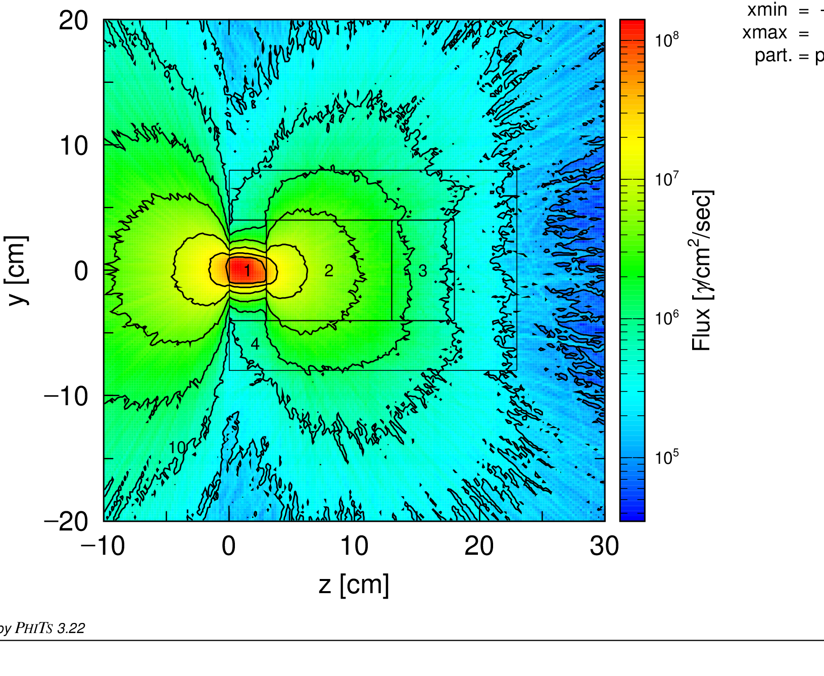
Fig. 4.13.17 xyz - Activated tungsten decay photon flux [\(\frac{\gamma}{\text{cm}^2\cdot\text{sec}}\)] in the target block

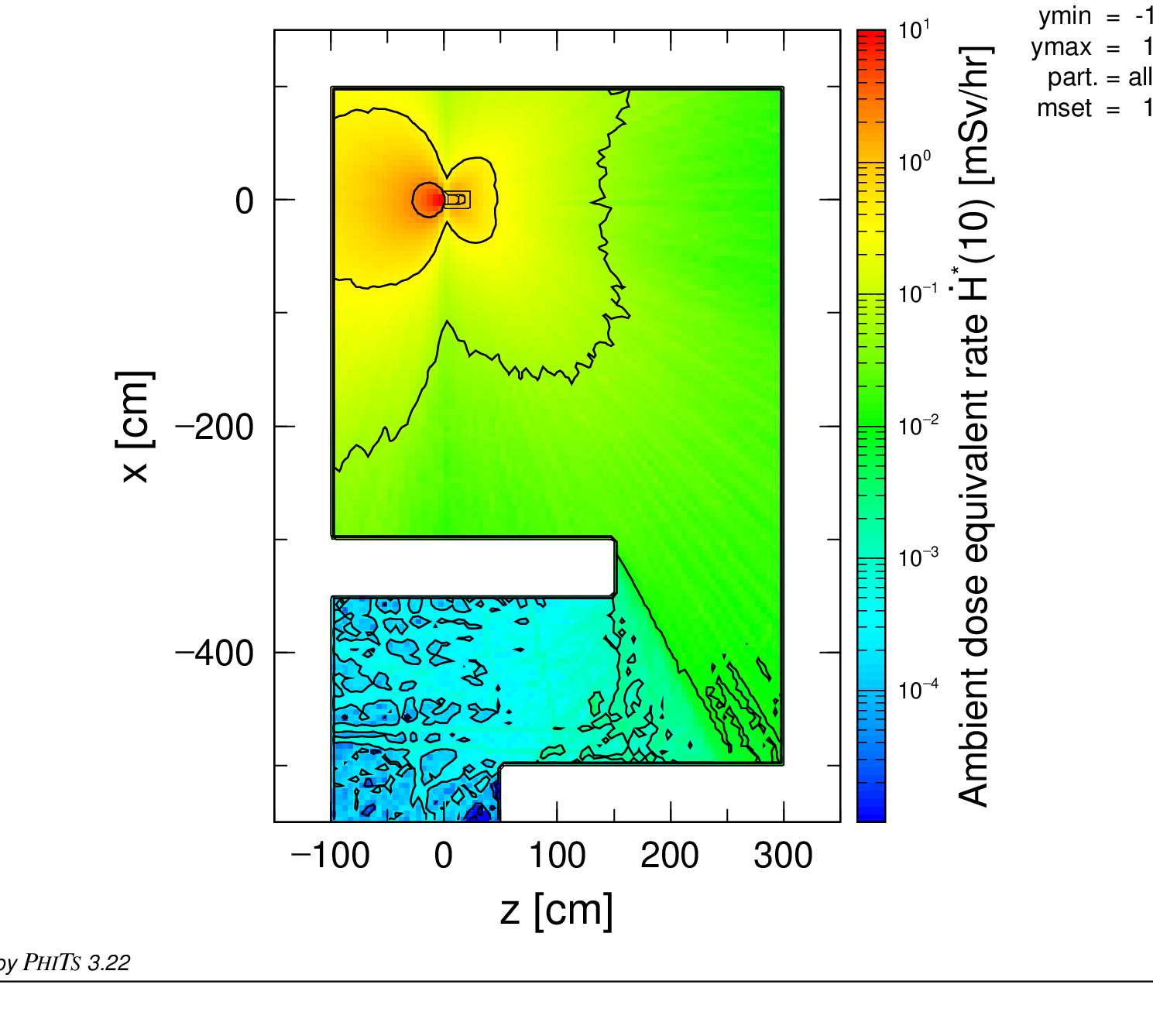
Fig. 4.13.18 xyz - \(\dot{H}^*(10)\) [mSv/hr] room map

Still, depending on your specific scenario, the mesh resolution, how concentrated or more evenly distributed the activation is, the mechanisms contributing to activation, what decay emissions are of concern, and what you wish to evaluate in a secondary PHITS simulation, setting totfact negative may yield improved results. For instance, in an object which is activated throughout but with increased activation in its core/center but is so large/dense that decay emissions would almost never escape from the center (perhaps a very thick cask which had previously held a strong neutron source), setting totfact negative would allow the more abundant voxels which are closer to the surface, but are less activated, to be sampled more often. If performing some dose assessment near this object, this would result in better statistics in the same amount of particle histories since fewer histories are “wasted” by spawning in the voxels in the smaller central region, which is the most activated but whose emissions almost never escape and contribute to the tally results. In general, the idea is to set the sign of totfact such that the number of particles contributing to your tallies of interest is maximized; though it is not always immediately obvious which sign results in more efficient use of computation time.