1.4. Tutorial example 2
Next example includes every important elements for minimum usage of ANGEL . If you have no time to have a read the following manual through, it is enough to learn this example for starting ANGEL . We show an input file and output graph in the following.
List 1.2 • Input of tutorial example 2
 1:  'Figure 2'                                          --- (1)
 2:  X: E (MeV)                                          --- (2)
 3:  Y: d\sigma/d\OmegadE (nb/MeV/sr)                    --- (3)
 4:  W:Comment = ^{12}C + ^{40}Ca/ X(1) Y(65)             --- (4)
 5:  A: X(4.3) Y(65) AX(5.5) AY(53)                      --- (5)
 6:  AW:Arrow/ X(4.5) Y(23) AX(4) AY(10)                 --- (6)
 7:  H:  X   Y(Histogram),DH0                            --- (7)
 8:      0.0    0
 9:      0.5   10
10:      1.5   20
11:      2.5   35
12:      3.5   30
13:      4.5   45
14:      5.5   70
15:      6.5    0
16:  H: X  Y(Spline),SL5                                 --- (8)
17:    0.5   40
18:    4     10
19:    6     20
20:    7     60
21:  H: X   DX    Y(Error bar),N3    D                   --- (9)
22:     2    1         50           10
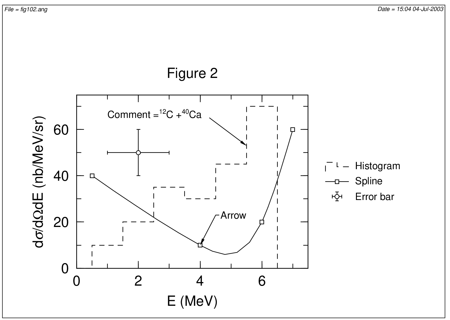
Fig. 1.2 Tutorial example 2
You can see a high quality image produced from a simple input by ANGEL . First, let me explain the points denoted by number in right-hand side of input lines in List 1.2.
- Title of graph
' 'The title of graph is specified between' '. This is shown in the middle upside the graph frame. The title can be removed and moved to horizontal direction by the parameter. - Title of X axis
X:The title of X axis is defined by the line started fromX:. You can use italic, bold, special characters, and other various expression of the characters in the title and also in any line of string. - Title of Y axis
Y:The title of Y axis is defned by the line started fromY:. - Comment
W:The comment in the figure is defined by the line started fromW:. The strings fromW:to/are shown in the figure at the point specified byX( ) Y( )as a comment. - Arrow
A:The arrow in the figure is defined by the line started fromA:. The start and end points of the arrow are specified byX( ) Y( )andAX( ) AY( ), respectively. - Arrow with Comment
AW:This is a combination of arrow and comment. The strings fromAW:to/are shown in the figure at the point specified byX( ) Y( )and the arrow is described toAX( ) AY( ).
In the following sections, we will explain another parameters which define the more detail of the above objects.
Next, we explain the basic section in ANGEL , H:, which defines the x-y graph. There are three H: sections (7), (8) and (9) in this example. The main purpose of this line of H: is to define the ordering of the following columns. As shown in the previous example, if the numerical data consist of x-value and y-value columns, we should write H: X Y. By this line, we can additionally define line type, symbol type, color, and legend.
The strings in the parenthesis after Y like Y(Histogram),DH0 are automatically shown in the right hand side of the graph frame as legends. The strings after the comma define the line type (D = Dashed Line, L = Solid Line, N = No Line), spline (S = Spline), histogram (H = Histogram), and symbol type (0 = No Symbol, 3 = Open Circle).
In the last section of (9), there are columns defined by DX, D. These define the error bars. DX defines the error bar of the X column, D defines the error bar of the Y column just before. In default, the value of the error is the same values around the y-value. It is explicitly expressed by D+-. If you want to define the different error values upper and lower values around the y-value, you should define those by different columns like D+ D-.
In ANGEL , we call ’section’ the part of the input file starting from alphabet characters with colon : like AW: H:.